[Porto Seguro] Porto Seguro Exploratory Analysis and Prediction

[공지사항] “출처: https://www.kaggle.com/code/jundthird/kor-exploratory-analysis-and-prediction”

Introduction

이 notebook은 다음의 커널들을 참고해 만들었습니다.

• Data Preparation and Exploration by Bert Carremans.
• Steering Whell of Fortune - Porto Seguro EDA by Heads or Tails
• Interactive Porto Insights - A Plot.ly Tutorial by Anisotropic
• Simple Stacker by Vladimir Demidov

Analysis packages

import pandas as pd
import numpy as np
import matplotlib.pyplot as plt
import seaborn as sns
from sklearn.utils import shuffle
from sklearn.preprocessing import PolynomialFeatures
from sklearn.preprocessing import StandardScaler
from sklearn.feature_selection import VarianceThreshold
from sklearn.feature_selection import SelectFromModel

from sklearn.model_selection import StratifiedKFold
from sklearn.model_selection import cross_val_score

from lightgbm import LGBMClassifier
from xgboost import XGBClassifier
from sklearn.linear_model import LogisticRegression

pd.set_option("display.max_columns", 100)

Load the data

trainset = pd.read_csv("./porto_seguro/train.csv")
testset = pd.read_csv("./porto_seguro/test.csv")

Few quick observations

이 대회에서의 데이터 설명을 통해 몇가지를 발견할 수 있습니다.

• 설명되어 있는 그룹이 거의 없으며 이러한 그룹들에 속한 feature들은 이름에 패턴을 포함하고 있습니다. (ind, reg, car, calc). ind는 개개인을 나타내고, reg는 등록여부, car는 따로 설명할 필요가 없고, calc는 계산된 필드를 암시할 것입니다
• 접미사 bin은 binary features
• 접미사 cat은 categorical features
• bin이나 cat이 없는 feature은 실수(연속형)나 정수(순서형)입니다
• 결측치는 -1입니다
• 우리가 예측해야할 변수는 target 칼럼입니다. 이는 피보험자의 보험 청구여부를 나타냅니다.

trainset.head()

	id	target	ps_ind_01	ps_ind_02_cat	ps_ind_03	ps_ind_04_cat	ps_ind_05_cat	ps_ind_06_bin	ps_ind_07_bin	ps_ind_08_bin	ps_ind_09_bin	ps_ind_10_bin	ps_ind_11_bin	ps_ind_12_bin	ps_ind_13_bin	ps_ind_14	ps_ind_15	ps_ind_16_bin	ps_ind_17_bin	ps_ind_18_bin	ps_reg_01	ps_reg_02	ps_reg_03	ps_car_01_cat	ps_car_02_cat	ps_car_03_cat	ps_car_04_cat	ps_car_05_cat	ps_car_06_cat	ps_car_07_cat	ps_car_08_cat	ps_car_09_cat	ps_car_10_cat	ps_car_11_cat	ps_car_11	ps_car_12	ps_car_13	ps_car_14	ps_car_15	ps_calc_01	ps_calc_02	ps_calc_03	ps_calc_04	ps_calc_05	ps_calc_06	ps_calc_07	ps_calc_08	ps_calc_09	ps_calc_10	ps_calc_11	ps_calc_12	ps_calc_13	ps_calc_14	ps_calc_15_bin	ps_calc_16_bin	ps_calc_17_bin	ps_calc_18_bin	ps_calc_19_bin	ps_calc_20_bin
0	7	0	2	2	5	1	0	0	1	0	0	0	0	0	0	0	11	0	1	0	0.7	0.2	0.718070	10	1	-1	0	1	4	1	0	0	1	12	2	0.400000	0.883679	0.370810	3.605551	0.6	0.5	0.2	3	1	10	1	10	1	5	9	1	5	8	0	1	1	0	0	1
1	9	0	1	1	7	0	0	0	0	1	0	0	0	0	0	0	3	0	0	1	0.8	0.4	0.766078	11	1	-1	0	-1	11	1	1	2	1	19	3	0.316228	0.618817	0.388716	2.449490	0.3	0.1	0.3	2	1	9	5	8	1	7	3	1	1	9	0	1	1	0	1	0
2	13	0	5	4	9	1	0	0	0	1	0	0	0	0	0	0	12	1	0	0	0.0	0.0	-1.000000	7	1	-1	0	-1	14	1	1	2	1	60	1	0.316228	0.641586	0.347275	3.316625	0.5	0.7	0.1	2	2	9	1	8	2	7	4	2	7	7	0	1	1	0	1	0
3	16	0	0	1	2	0	0	1	0	0	0	0	0	0	0	0	8	1	0	0	0.9	0.2	0.580948	7	1	0	0	1	11	1	1	3	1	104	1	0.374166	0.542949	0.294958	2.000000	0.6	0.9	0.1	2	4	7	1	8	4	2	2	2	4	9	0	0	0	0	0	0
4	17	0	0	2	0	1	0	1	0	0	0	0	0	0	0	0	9	1	0	0	0.7	0.6	0.840759	11	1	-1	0	-1	14	1	1	2	1	82	3	0.316070	0.565832	0.365103	2.000000	0.4	0.6	0.0	2	2	6	3	10	2	12	3	1	1	3	0	0	0	1	1	0

정말로 cat이 접미사로 붙은 feature들은 범주형이고, 정수값은 0에서 n까지, bin feature들은 0 혹은 1의 값을 가지는 것을 확인할 수 있습니다.

데이터 세트의 shape을 확인해봅니다.

print("Train dataset (rows, cols):",trainset.shape, "\nTest dataset (rows, cols):",testset.shape)

Train dataset (rows, cols): (595212, 59) 
Test dataset (rows, cols): (892816, 58)

칼럼의 개수가 차이나는 이유는 target 칼럼의 유무

print("Columns in train and not in test dataset:",set(trainset.columns)-set(testset.columns))

Columns in train and not in test dataset: {'target'}

Introduction of metadata

데이터 다루는 것을 쉽게 하기 위하여, 변수들에 대한 meta-information을 담은 데이터프레임을 만들어줍니다. 이는 다양한 변수를 가진 feature들의 조사, 검사, 모델링하는데 용이하게 해줍니다.

메타데이터로 사용할 것들:

• use: input, ID, target
• type: nominal, interval, ordinal, binary
• preserve: True or False
• dataType: int, float, char
• category: ind, reg, car, calc

data = []
for feature in trainset.columns:
    # Defining the role
    if feature == "target":
        use = "target"
    elif feature == "id":
        use = "id"
    else:
        use = "input"
        
    # Defining the type
    if "bin" in feature or feature == "target":
        type = "binary"
    elif "cat" in feature or feature == "id":
        type = "categorical"
    elif np.issubdtype(trainset[feature].dtype, np.floating):
        type = "real"
    elif np.issubdtype(trainset[feature].dtype, np.integer):
        type = "integer"
        
    # id를 제외하고 모든 변수들을 preverse = Ture로 설정
    preserve = True
    if feature == "id":
        preserve = False
        
    # Defining the data type
    dtype = trainset[feature].dtype
    
    category = "none"
    # Defining the category
    if "ind" in feature:
        category = "individual"
    elif "reg" in feature:
        category = "registration"
    elif "car" in feature:
        category = "car"
    elif "calc" in feature:
        category = "calculated"
        
    feature_dictionary = {
        'varname': feature,
        'use': use,
        'type': type,
        'preserve': preserve,
        'dtype': dtype,
        'category' : category
    }
    
    data.append(feature_dictionary)
    
metadata = pd.DataFrame(data, columns=['varname', 'use', 'type', 'preserve', 'dtype', 'category'])
metadata.set_index("varname", inplace=True)
metadata

	use	type	preserve	dtype	category
varname
id	id	categorical	False	int64	none
target	target	binary	True	int64	none
ps_ind_01	input	integer	True	int64	individual
ps_ind_02_cat	input	categorical	True	int64	individual
ps_ind_03	input	integer	True	int64	individual
ps_ind_04_cat	input	categorical	True	int64	individual
ps_ind_05_cat	input	categorical	True	int64	individual
ps_ind_06_bin	input	binary	True	int64	individual
ps_ind_07_bin	input	binary	True	int64	individual
ps_ind_08_bin	input	binary	True	int64	individual
ps_ind_09_bin	input	binary	True	int64	individual
ps_ind_10_bin	input	binary	True	int64	individual
ps_ind_11_bin	input	binary	True	int64	individual
ps_ind_12_bin	input	binary	True	int64	individual
ps_ind_13_bin	input	binary	True	int64	individual
ps_ind_14	input	integer	True	int64	individual
ps_ind_15	input	integer	True	int64	individual
ps_ind_16_bin	input	binary	True	int64	individual
ps_ind_17_bin	input	binary	True	int64	individual
ps_ind_18_bin	input	binary	True	int64	individual
ps_reg_01	input	real	True	float64	registration
ps_reg_02	input	real	True	float64	registration
ps_reg_03	input	real	True	float64	registration
ps_car_01_cat	input	categorical	True	int64	car
ps_car_02_cat	input	categorical	True	int64	car
ps_car_03_cat	input	categorical	True	int64	car
ps_car_04_cat	input	categorical	True	int64	car
ps_car_05_cat	input	categorical	True	int64	car
ps_car_06_cat	input	categorical	True	int64	car
ps_car_07_cat	input	categorical	True	int64	car
ps_car_08_cat	input	categorical	True	int64	car
ps_car_09_cat	input	categorical	True	int64	car
ps_car_10_cat	input	categorical	True	int64	car
ps_car_11_cat	input	categorical	True	int64	car
ps_car_11	input	integer	True	int64	car
ps_car_12	input	real	True	float64	car
ps_car_13	input	real	True	float64	car
ps_car_14	input	real	True	float64	car
ps_car_15	input	real	True	float64	car
ps_calc_01	input	real	True	float64	calculated
ps_calc_02	input	real	True	float64	calculated
ps_calc_03	input	real	True	float64	calculated
ps_calc_04	input	integer	True	int64	calculated
ps_calc_05	input	integer	True	int64	calculated
ps_calc_06	input	integer	True	int64	calculated
ps_calc_07	input	integer	True	int64	calculated
ps_calc_08	input	integer	True	int64	calculated
ps_calc_09	input	integer	True	int64	calculated
ps_calc_10	input	integer	True	int64	calculated
ps_calc_11	input	integer	True	int64	calculated
ps_calc_12	input	integer	True	int64	calculated
ps_calc_13	input	integer	True	int64	calculated
ps_calc_14	input	integer	True	int64	calculated
ps_calc_15_bin	input	binary	True	int64	calculated
ps_calc_16_bin	input	binary	True	int64	calculated
ps_calc_17_bin	input	binary	True	int64	calculated
ps_calc_18_bin	input	binary	True	int64	calculated
ps_calc_19_bin	input	binary	True	int64	calculated
ps_calc_20_bin	input	binary	True	int64	calculated

예를 들어, 아래와 같이 모든 범주형 변수들을 확인할 수 있습니다.

metadata[(metadata.type == "categorical") & (metadata.preserve)].index

Index(['ps_ind_02_cat', 'ps_ind_04_cat', 'ps_ind_05_cat', 'ps_car_01_cat',
       'ps_car_02_cat', 'ps_car_03_cat', 'ps_car_04_cat', 'ps_car_05_cat',
       'ps_car_06_cat', 'ps_car_07_cat', 'ps_car_08_cat', 'ps_car_09_cat',
       'ps_car_10_cat', 'ps_car_11_cat'],
      dtype='object', name='varname')

category 값들이 몇개인지 확인해봅시다.

pd.DataFrame({"count": metadata.groupby(["category"])["category"].size()}).reset_index()

	category	count
0	calculated	20
1	car	16
2	individual	18
3	none	2
4	registration	3

이번엔 use와 type의 값들이 몇개인지 확인

pd.DataFrame({"count": metadata.groupby(["use", "type"])["use"].size()}).reset_index()

	use	type	count
0	id	categorical	1
1	input	binary	17
2	input	categorical	14
3	input	integer	16
4	input	real	10
5	target	binary	1

Data analysis and statistics

Target variable

plt.figure()
fig, ax = plt.subplots(figsize=(6, 6))
x = trainset["target"].value_counts().index.values
y = trainset["target"].value_counts().values

sns.barplot(ax=ax, x=x, y=y)
plt.ylabel('Number of values', fontsize=12)
plt.xlabel('Target value', fontsize=12)
plt.tick_params(axis="both", which="major", labelsize=12)
plt.show()

<Figure size 2400x1500 with 0 Axes>

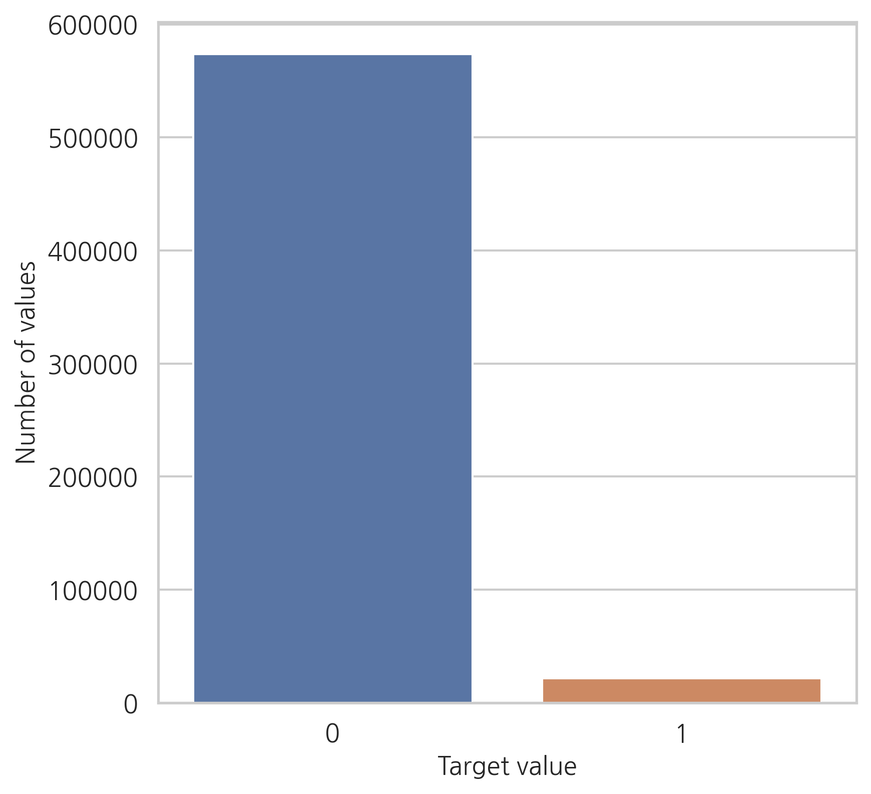
오직 target 값의 3.64%만 1의 값을 가지고 있습니다. 데이터가 매우 불균형하다는 의미. 따라서, target=0을 undersampling을 하거나 target=1을 oversampling할 수 있습니다. (데이터 세트가 매우 크기 때문에, 여기서는 target=0을 undersampling합니다)

Real features

variable = metadata[(metadata.type == "real") & (metadata.preserve)].index
trainset[variable].describe()

	ps_reg_01	ps_reg_02	ps_reg_03	ps_car_12	ps_car_13	ps_car_14	ps_car_15	ps_calc_01	ps_calc_02	ps_calc_03
count	595212.000000	595212.000000	595212.000000	595212.000000	595212.000000	595212.000000	595212.000000	595212.000000	595212.000000	595212.000000
mean	0.610991	0.439184	0.551102	0.379945	0.813265	0.276256	3.065899	0.449756	0.449589	0.449849
std	0.287643	0.404264	0.793506	0.058327	0.224588	0.357154	0.731366	0.287198	0.286893	0.287153
min	0.000000	0.000000	-1.000000	-1.000000	0.250619	-1.000000	0.000000	0.000000	0.000000	0.000000
25%	0.400000	0.200000	0.525000	0.316228	0.670867	0.333167	2.828427	0.200000	0.200000	0.200000
50%	0.700000	0.300000	0.720677	0.374166	0.765811	0.368782	3.316625	0.500000	0.400000	0.500000
75%	0.900000	0.600000	1.000000	0.400000	0.906190	0.396485	3.605551	0.700000	0.700000	0.700000
max	0.900000	1.800000	4.037945	1.264911	3.720626	0.636396	3.741657	0.900000	0.900000	0.900000

pow(trainset["ps_car_12"]*10, 2)

0         16.00
1         10.00
2         10.00
3         14.00
4          9.99
          ...  
595207    14.00
595208    15.00
595209    15.80
595210    14.00
595211    16.00
Name: ps_car_12, Length: 595212, dtype: float64

(pow(trainset['ps_car_15'],2)).head(10)

0    13.0
1     6.0
2    11.0
3     4.0
4     4.0
5     9.0
6    10.0
7    11.0
8     8.0
9    13.0
Name: ps_car_15, dtype: float64

Features with missing values

ps_reg_03, ps_car_12, ps_car_14는 결측치를 가지고 있습니다. (minimum 값이 -1)

Registration features

ps_reg_01, ps_reg_02는 분모를 10으로 가지는 분수입니다. (0,1, 0.2, 0.3

Car features

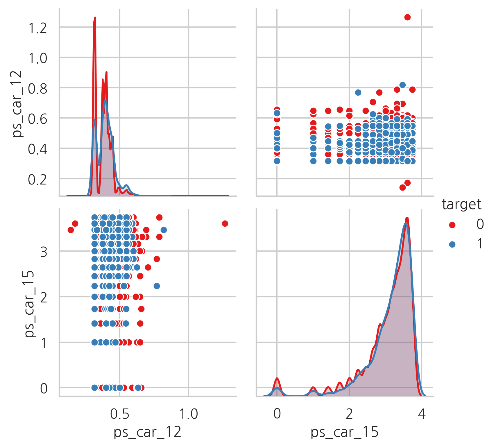
ps_car_12는 (몇몇은 근사치) 자연수의 제곱근(10으로 나눈 값)입니다
ps_car_15는 자연수의 제곱근입니다. pairplot을 통해 값들을 시각화해봅시다

sample = trainset.sample(frac=0.05)
var = ["ps_car_12", "ps_car_15", "target"]
sample = sample[var]
sns.pairplot(sample, hue="target", palette="Set1", diag_kind="kde")
plt.show()

Calculated features

ps_calc_01, ps_calc_02, ps_calc_03은 매우 비슷한 분포를 가지고 있고, 모든 maximum 값이 0.9이기 때문에 일종의 비율일 수도 있습니다. 다른 calc 칼럼은 최댓값이 정수형입니다. (5, 6, 7, 10, 12)

density plot을 이용하여 real feature을 시각화해봅니다.

var = metadata[(metadata.type == "real") & (metadata.preserve)].index
i = 0
t1 = trainset.loc[trainset["target"] == 1]
t0 = trainset.loc[trainset["target"] == 0]

sns.set_style("whitegrid")
plt.figure()
fig, ax = plt.subplots(3, 4, figsize=(16, 12))

for feature in var:
    i += 1
    plt.subplot(3, 4, i)
    sns.kdeplot(t1[feature], bw=0.5, label="target = 1")
    sns.kdeplot(t0[feature], bw=0.5, label="target = 0")
    plt.ylabel("Density plot", fontsize=12)
    plt.xlabel(feature, fontsize=12)
    plt.tick_params(axis="both", which="major", labelsize=12)
plt.show()

<Figure size 2400x1500 with 0 Axes>

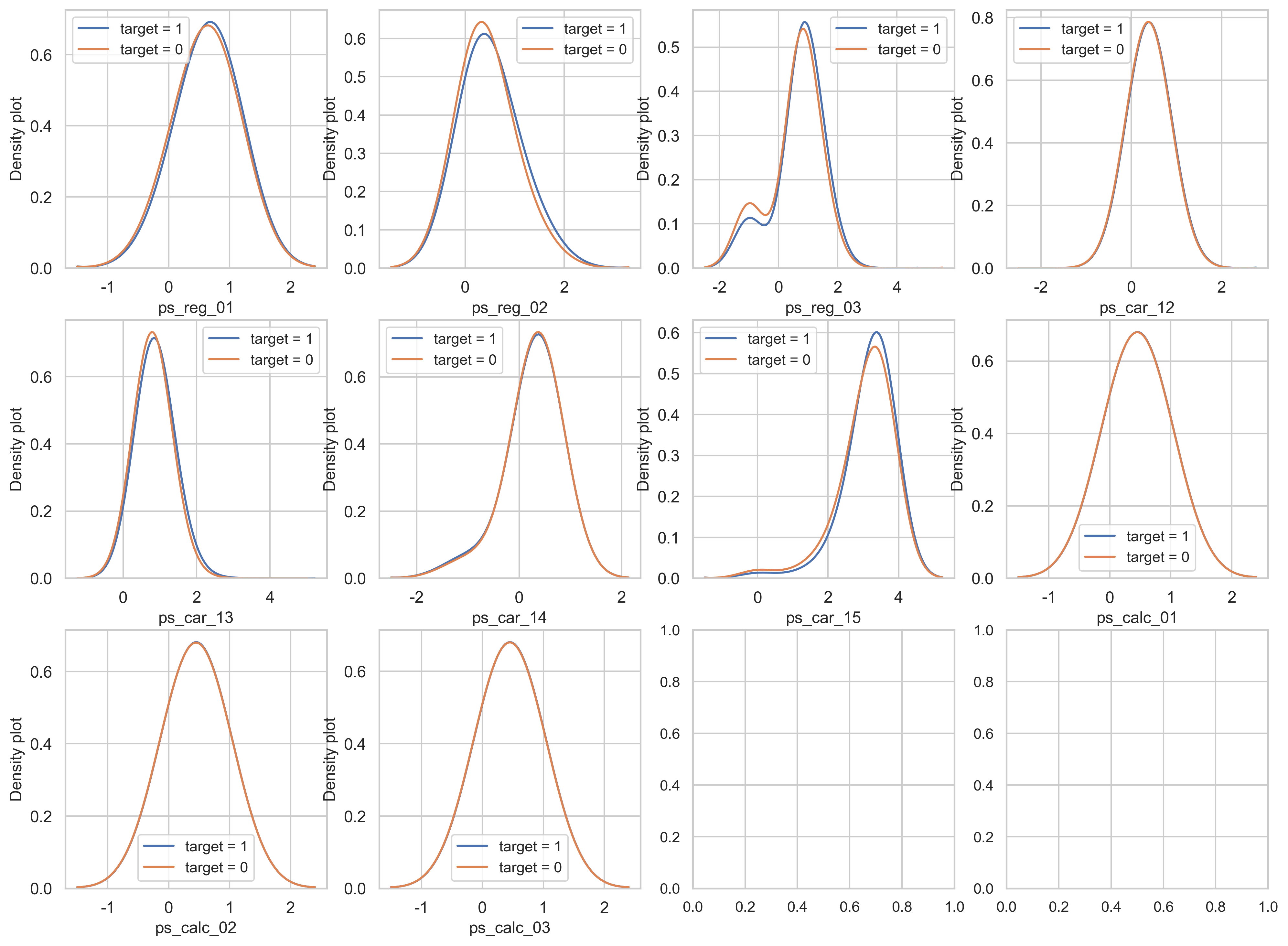
ps_reg_02, ps_car_13, ps_car_15는 target=0과 target=1과 관련된 값들 중 가장 다른 분포를 나타냅니다.

이제 상관관계를 시각화해봅시다.

def corr_heatmap(var):
    correlations = trainset[var].corr()
    
    cmap = sns.diverging_palette(50, 10, as_cmap=True)
    fig, ax = plt.subplots(figsize=(10, 10))
    sns.heatmap(correlations, cmap=cmap, vmax=1.0, center=0, fmt=".2f",
                square=True, linewidths=.5, annot=True, cbar_kws={"shrink": .75})
    plt.show()
    
var = metadata[(metadata.type == "real") & (metadata.preserve)].index
corr_heatmap(var)

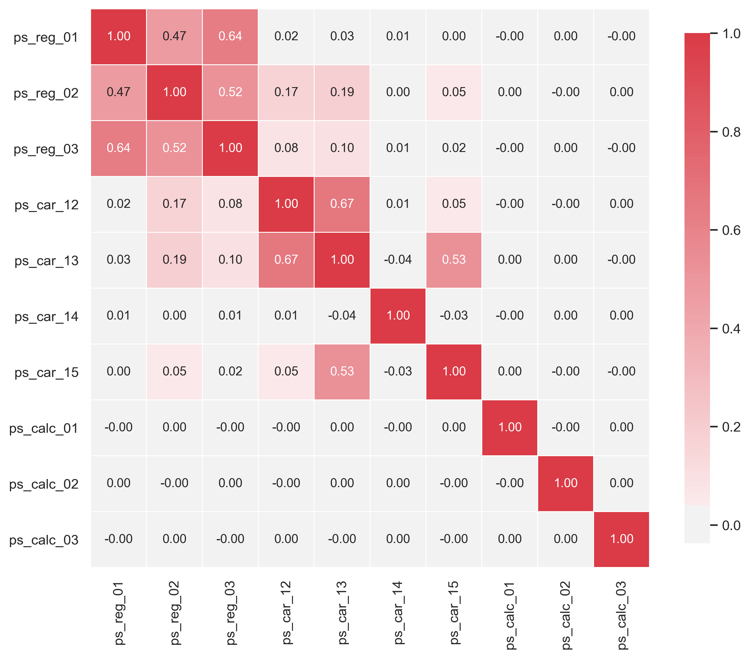
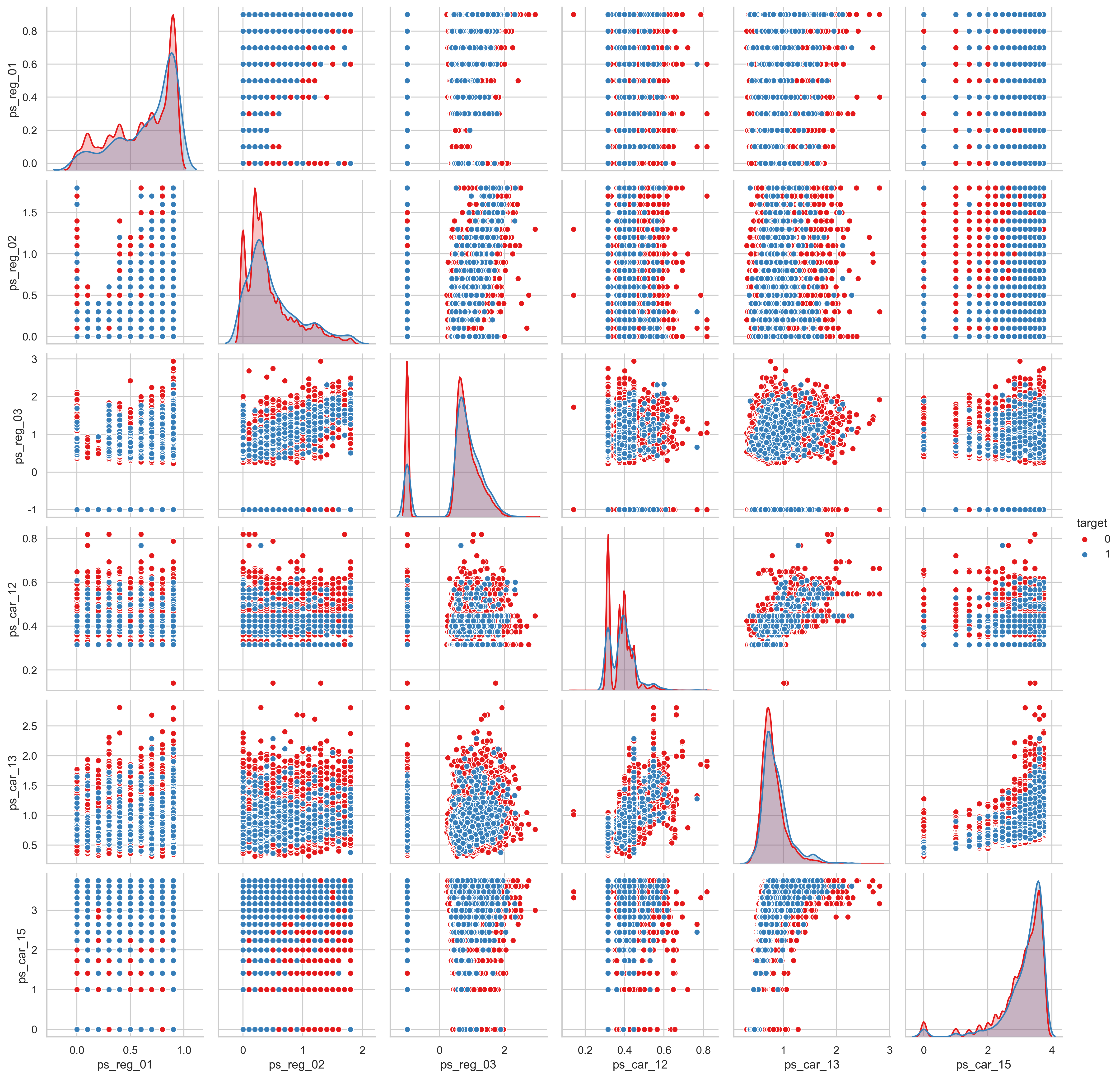
몇몇은 강한 상관관계를 보입니다:

• ps_reg_01 with ps_reg_02 (0.47);
• ps_reg_01 with ps_reg_03 (0.64);
• ps_reg_02 with ps_reg_03 (0.52);
• ps_car_12 with ps_car_13 (0.67);
• ps_car_13 with ps_car_15 (0.53);

상관관계가 있는 값들의 나타내기 위해 pairplot을 사용합니다.

sample = trainset.sample(frac=0.05)
var = ['ps_reg_01', 'ps_reg_02', 'ps_reg_03', 'ps_car_12', 'ps_car_13', 'ps_car_15', 'target']
sample = sample[var]
sns.pairplot(sample, hue="target", palette="Set1", diag_kind="kde")
plt.show()

Binary features

v = metadata[(metadata.type == "binary") & (metadata.preserve)].index
trainset[v].describe()

	target	ps_ind_06_bin	ps_ind_07_bin	ps_ind_08_bin	ps_ind_09_bin	ps_ind_10_bin	ps_ind_11_bin	ps_ind_12_bin	ps_ind_13_bin	ps_ind_16_bin	ps_ind_17_bin	ps_ind_18_bin	ps_calc_15_bin	ps_calc_16_bin	ps_calc_17_bin	ps_calc_18_bin	ps_calc_19_bin	ps_calc_20_bin
count	595212.000000	595212.000000	595212.000000	595212.000000	595212.000000	595212.000000	595212.000000	595212.000000	595212.000000	595212.000000	595212.000000	595212.000000	595212.000000	595212.000000	595212.000000	595212.000000	595212.000000	595212.000000
mean	0.036448	0.393742	0.257033	0.163921	0.185304	0.000373	0.001692	0.009439	0.000948	0.660823	0.121081	0.153446	0.122427	0.627840	0.554182	0.287182	0.349024	0.153318
std	0.187401	0.488579	0.436998	0.370205	0.388544	0.019309	0.041097	0.096693	0.030768	0.473430	0.326222	0.360417	0.327779	0.483381	0.497056	0.452447	0.476662	0.360295
min	0.000000	0.000000	0.000000	0.000000	0.000000	0.000000	0.000000	0.000000	0.000000	0.000000	0.000000	0.000000	0.000000	0.000000	0.000000	0.000000	0.000000	0.000000
25%	0.000000	0.000000	0.000000	0.000000	0.000000	0.000000	0.000000	0.000000	0.000000	0.000000	0.000000	0.000000	0.000000	0.000000	0.000000	0.000000	0.000000	0.000000
50%	0.000000	0.000000	0.000000	0.000000	0.000000	0.000000	0.000000	0.000000	0.000000	1.000000	0.000000	0.000000	0.000000	1.000000	1.000000	0.000000	0.000000	0.000000
75%	0.000000	1.000000	1.000000	0.000000	0.000000	0.000000	0.000000	0.000000	0.000000	1.000000	0.000000	0.000000	0.000000	1.000000	1.000000	1.000000	1.000000	0.000000
max	1.000000	1.000000	1.000000	1.000000	1.000000	1.000000	1.000000	1.000000	1.000000	1.000000	1.000000	1.000000	1.000000	1.000000	1.000000	1.000000	1.000000	1.000000

binary feature의 분포를 시각화

bin_col = [col for col in trainset.columns if "_bin" in col]
zero_list = []
one_list = []
for col in bin_col:
    zero_list.append((trainset[col] == 0).sum() / trainset.shape[0] * 100)
    one_list.append((trainset[col] == 1).sum() / trainset.shape[0] * 100)
plt.figure()
fig, ax = plt.subplots(figsize=(6, 6))

# Barplot
p1 = sns.barplot(ax=ax, x=bin_col, y=zero_list, color="blue")
p2 = sns.barplot(ax=ax, x=bin_col, y=one_list, bottom=zero_list, color="red")
plt.ylabel("Percent of zero/one [%]", fontsize=12)
plt.xlabel("Binary features", fontsize=12)
locs, labels = plt.xticks()
plt.setp(labels, rotation=90)
plt.tick_params(axis="both", which="major", labelsize=12)
plt.legend((p1, p2), ("Zero", "One"))
plt.show()

<Figure size 2400x1500 with 0 Axes>

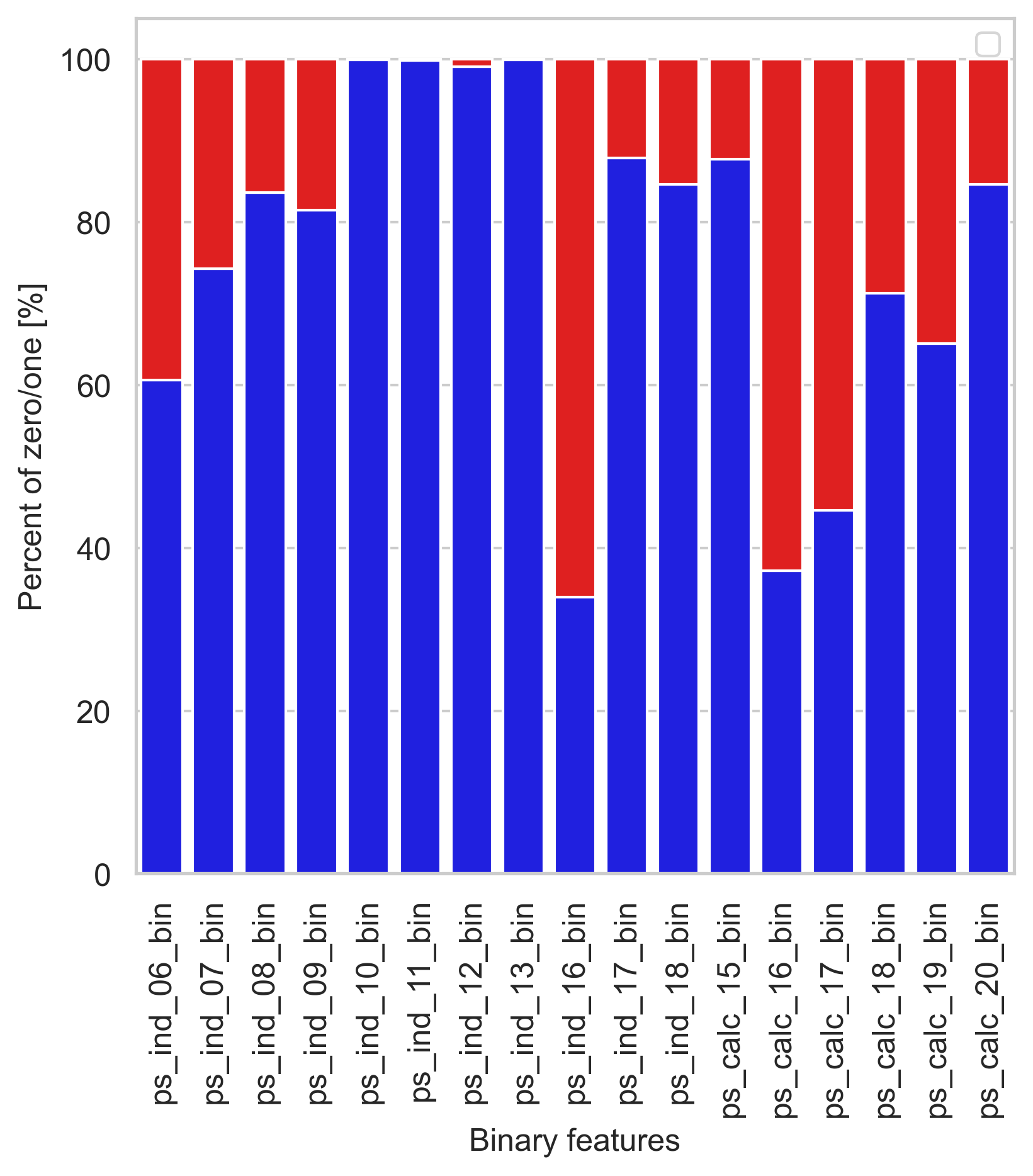
ps_ind_10_bin, ps_ind_11_bin, ps_ind_12_bin, ps_ind_13_bin 칼럼들은 매우 적은 비율의 1 값을 가지고 있습니다. (0.5% 미만) 반면에, ps_ind_16_bin, ps_calcs_16_bin 칼럼들은 큰 비율의 1 값을 가지고 있습니다. (60% 이상)

이제 target 값에 해당하는 binary 데이터의 분포를 살펴봅시다.

var = metadata[(metadata.type == "binary") & (metadata.preserve)].index
var = [col for col in trainset.columns if "_bin" in col]
i = 0
t1 = trainset.loc[trainset["target"] != 0]
t0 = trainset.loc[trainset["target"] == 0]

sns.set_style("whitegrid")
plt.figure()
fig, ax = plt.subplots(6, 3, figsize=(12, 24))

for feature in var:
    i += 1
    plt.subplot(6, 3, i)
    sns.kdeplot(t1[feature], bw=0.5, label="target = 1")
    sns.kdeplot(t0[feature], bw=0.5, label="target = 0")
    plt.ylabel("Density plot", fontsize=12)
    plt.xlabel(feature, fontsize=12)
    plt.tick_params(axis="both", which="major", labelsize=12)
plt.show()

<Figure size 2400x1500 with 0 Axes>

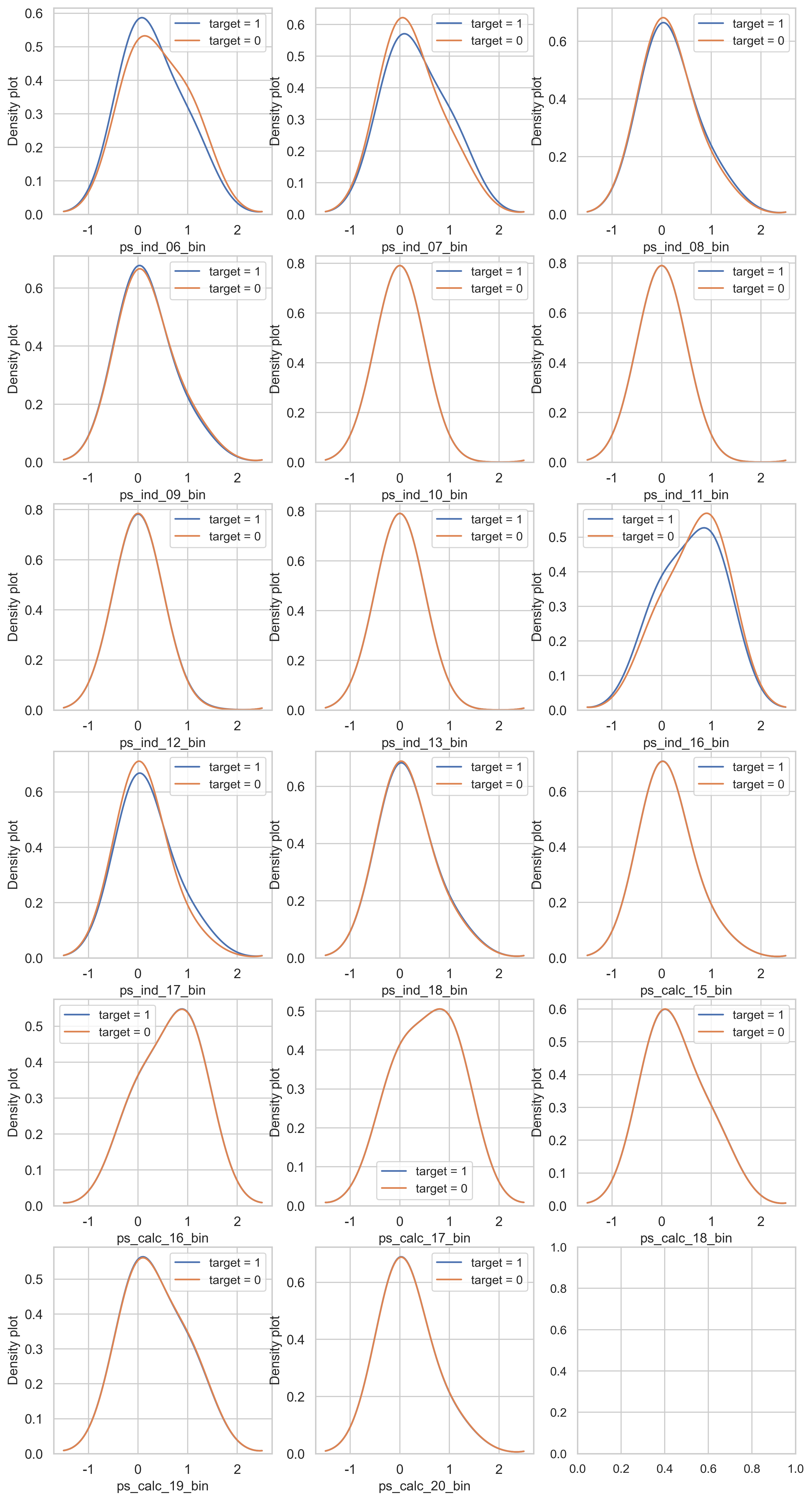
ps_ind_06_bin, ps_ind_07_bin, ps_ind_16_bin, ps_ind_17_bin 칼럼들은 target 값에 따른 데이터 분포가 불균형하다. 반면에 ps_ind_08_bin은 데이터 불균형이 적습니다. 반면에 다른 칼럼들은 꽤 데이터가 균형잡힌 모습입니다.

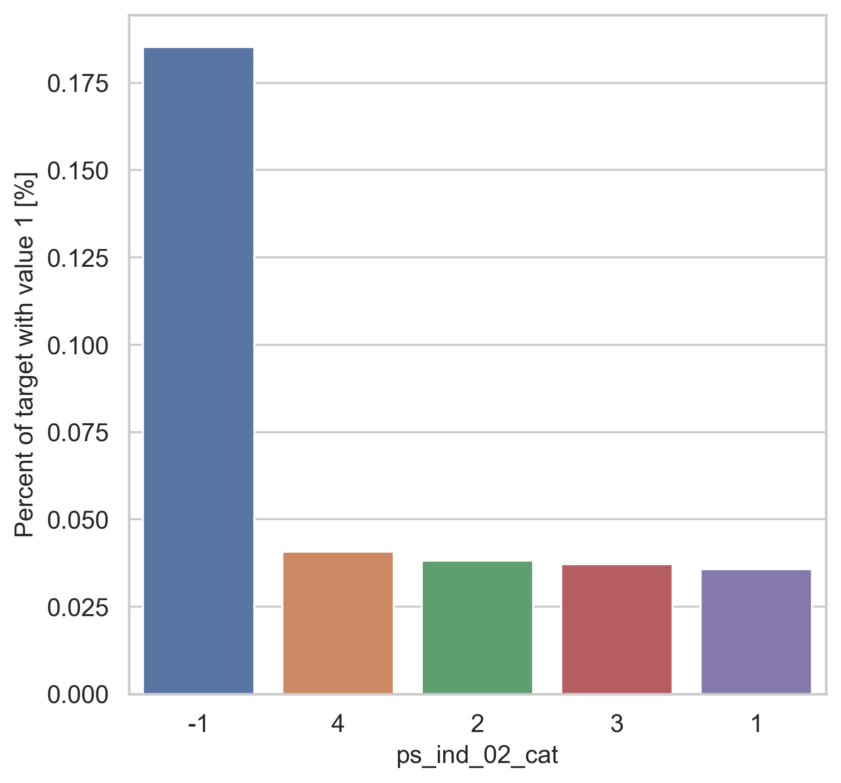
Categorical features

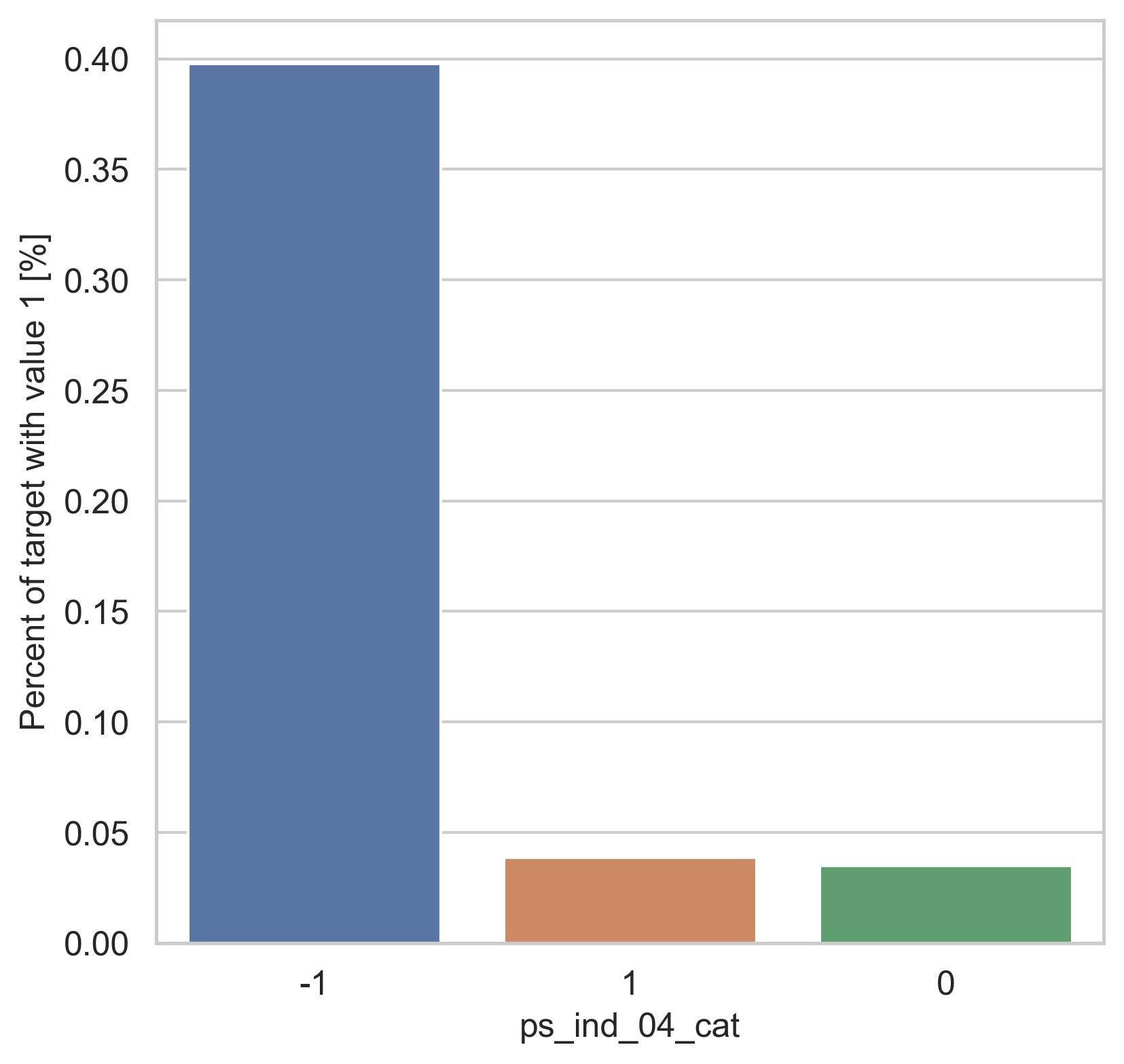
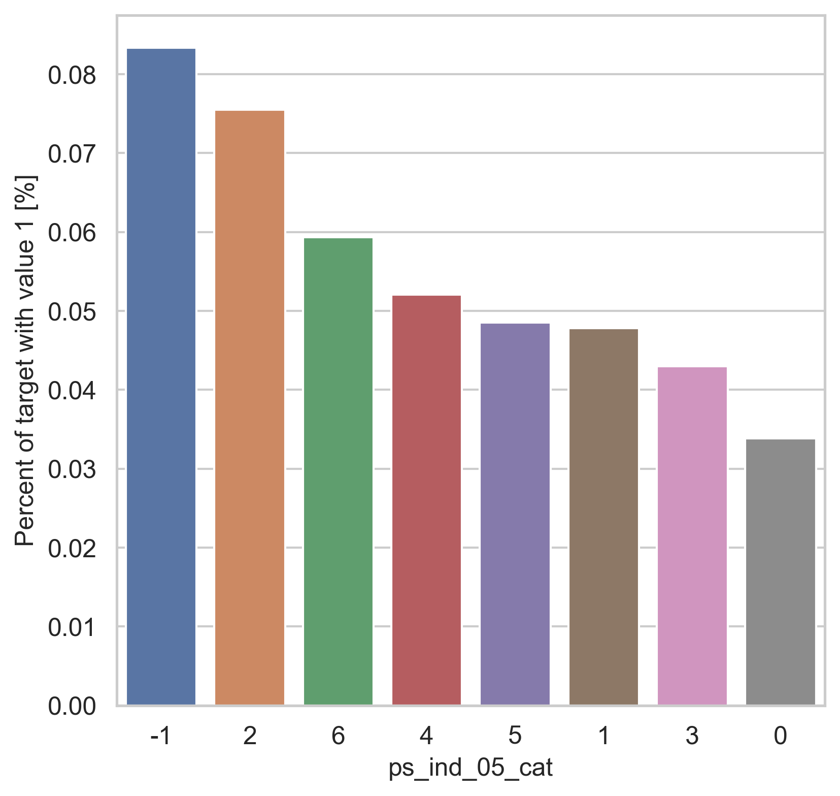
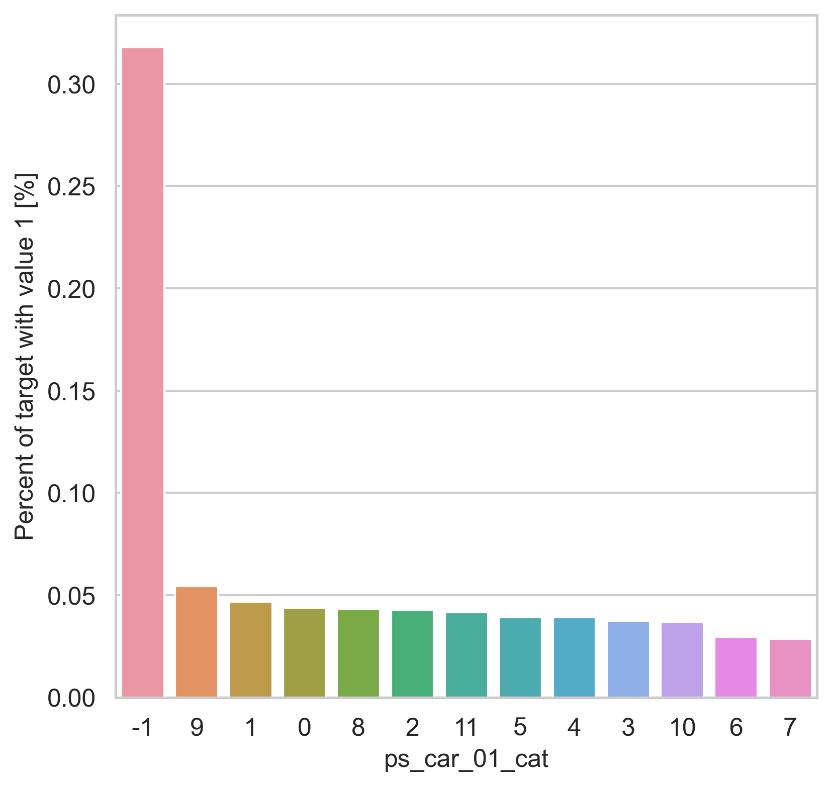
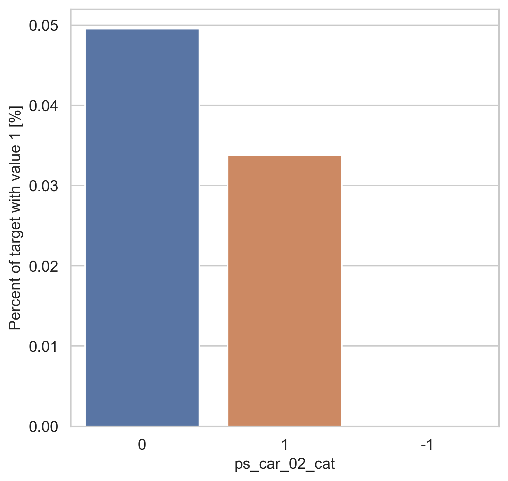
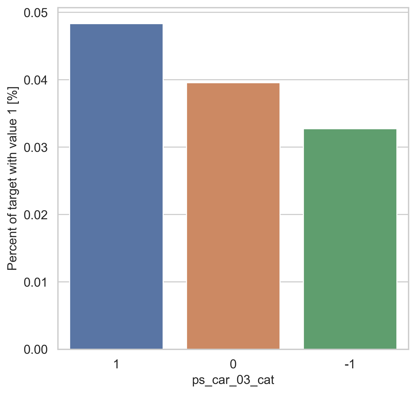
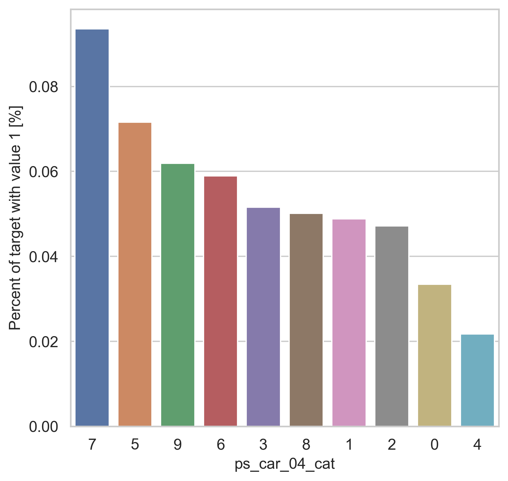
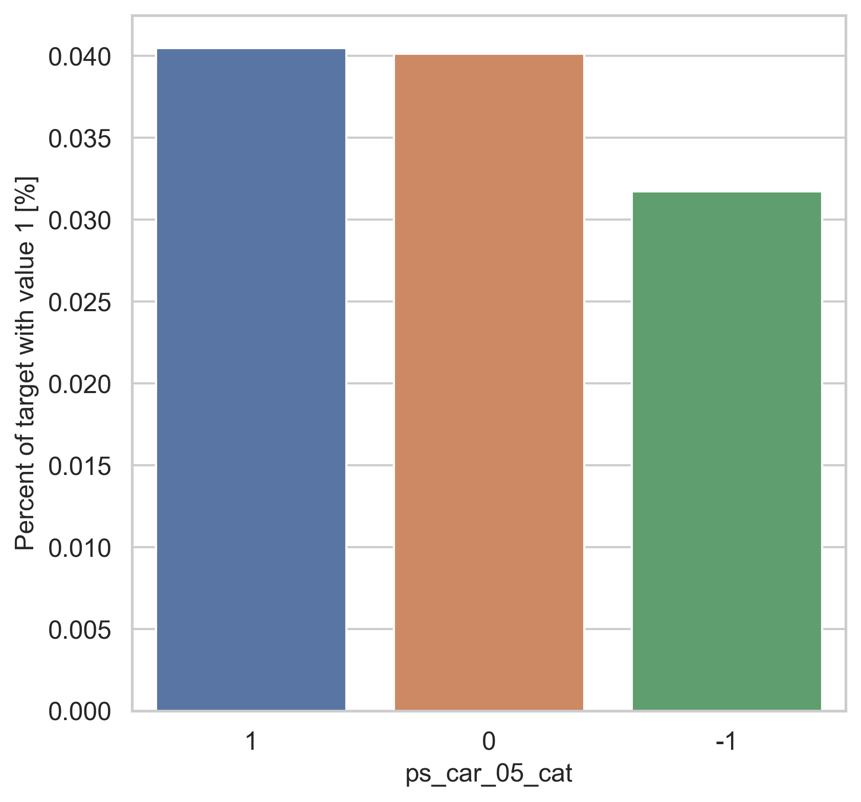
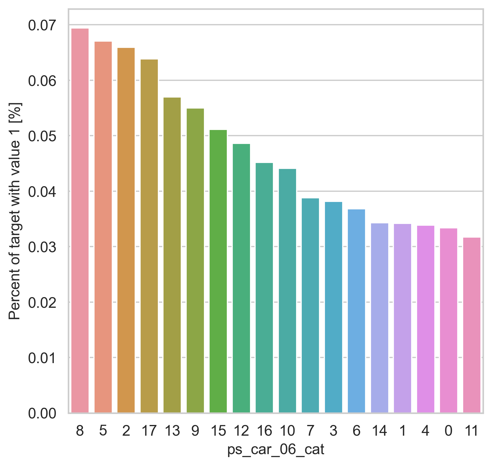
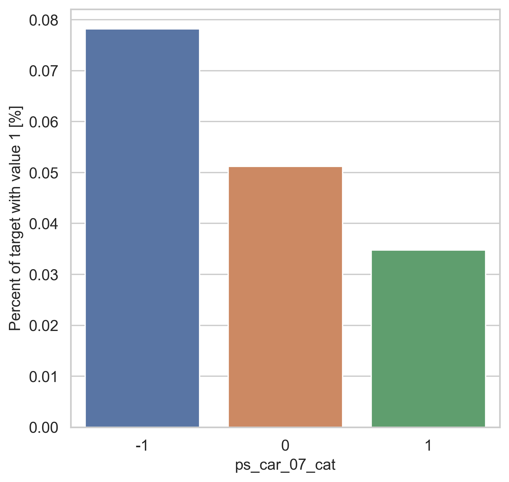
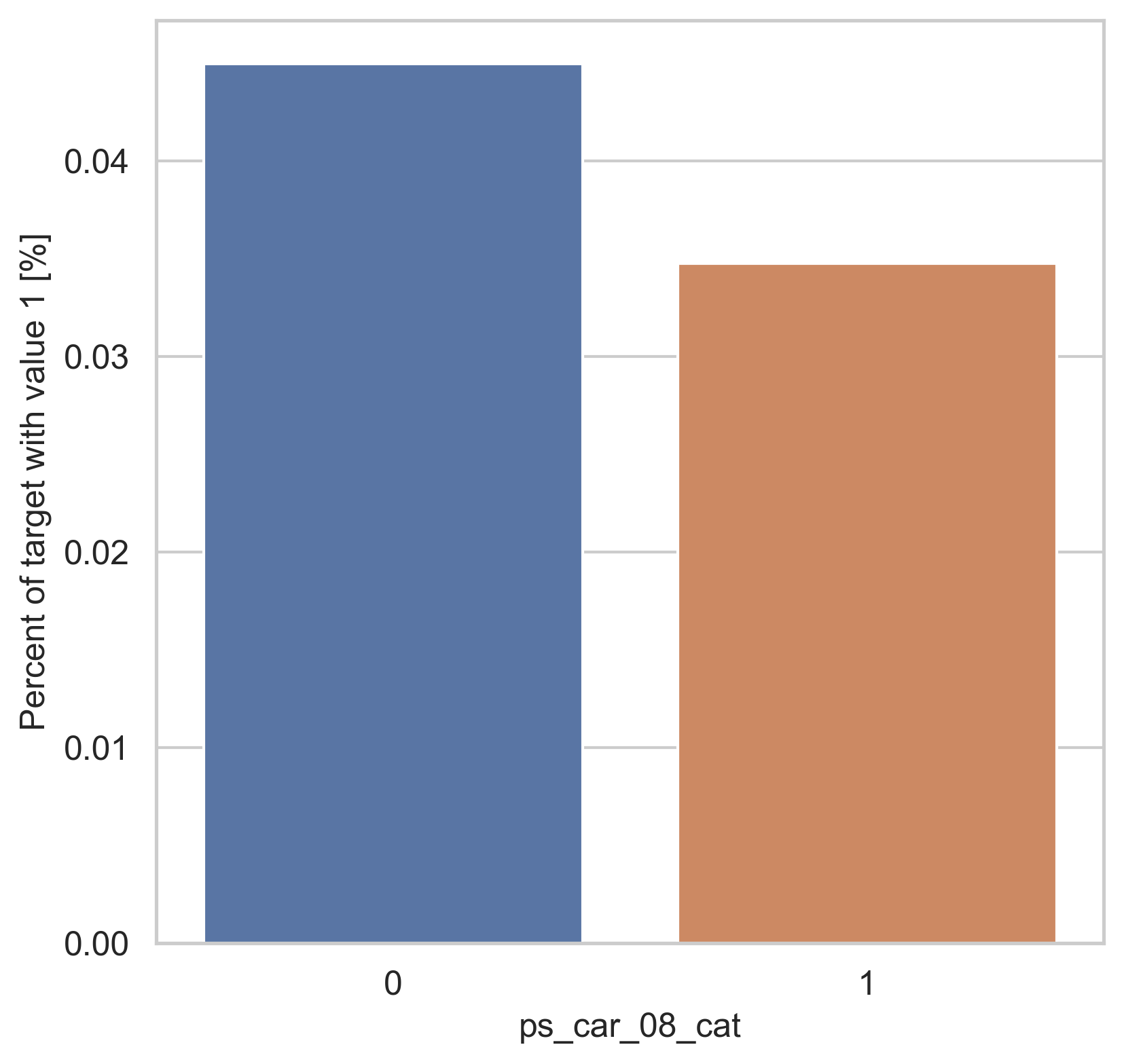
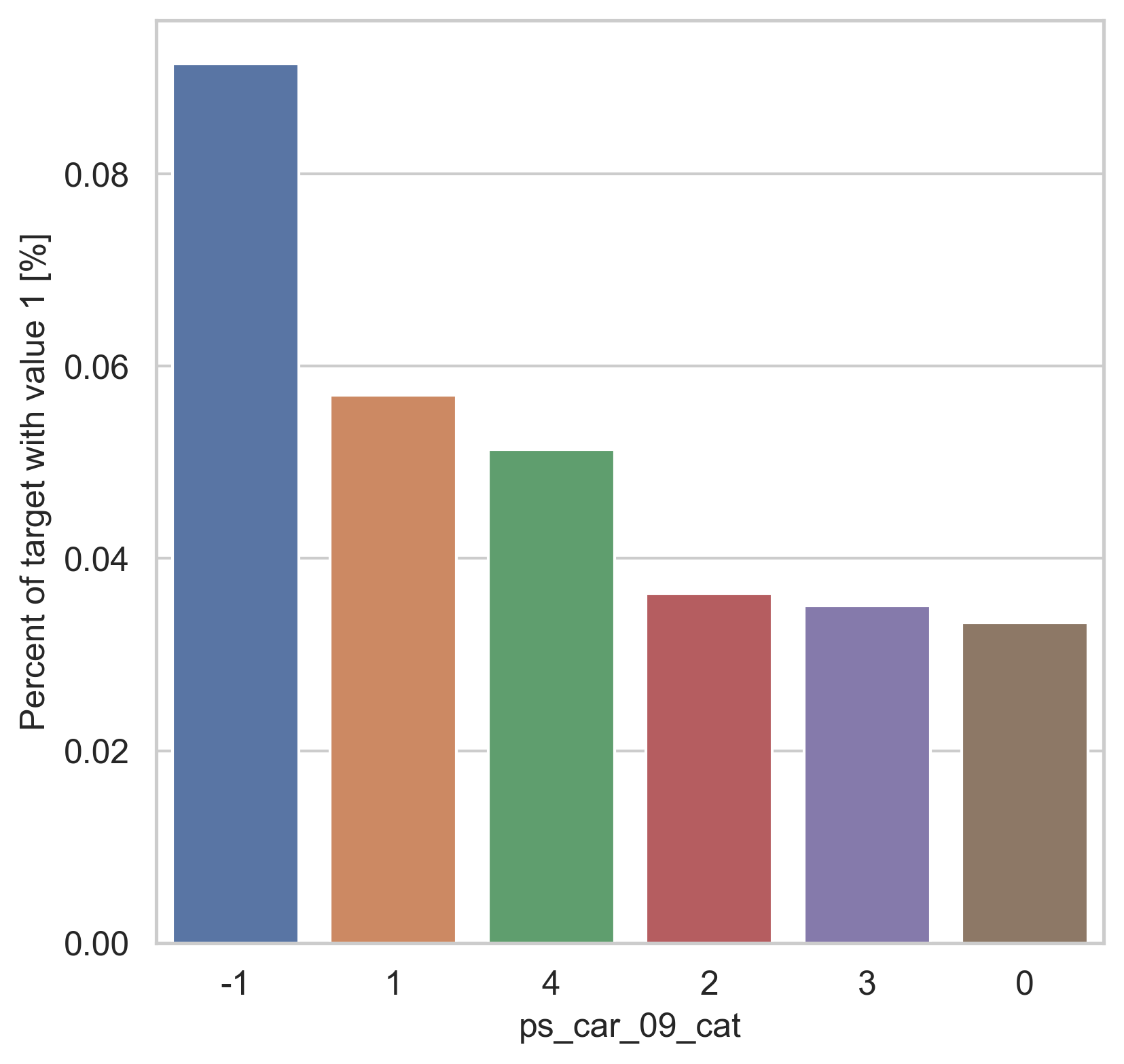
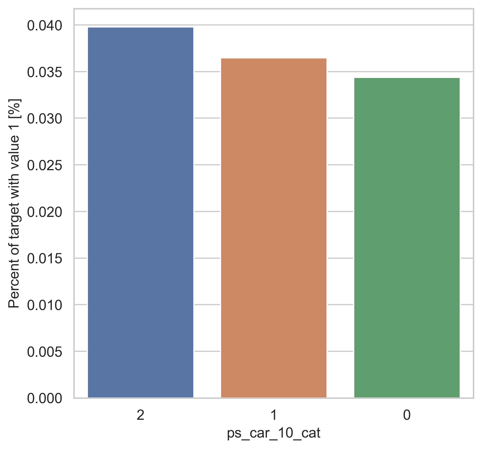
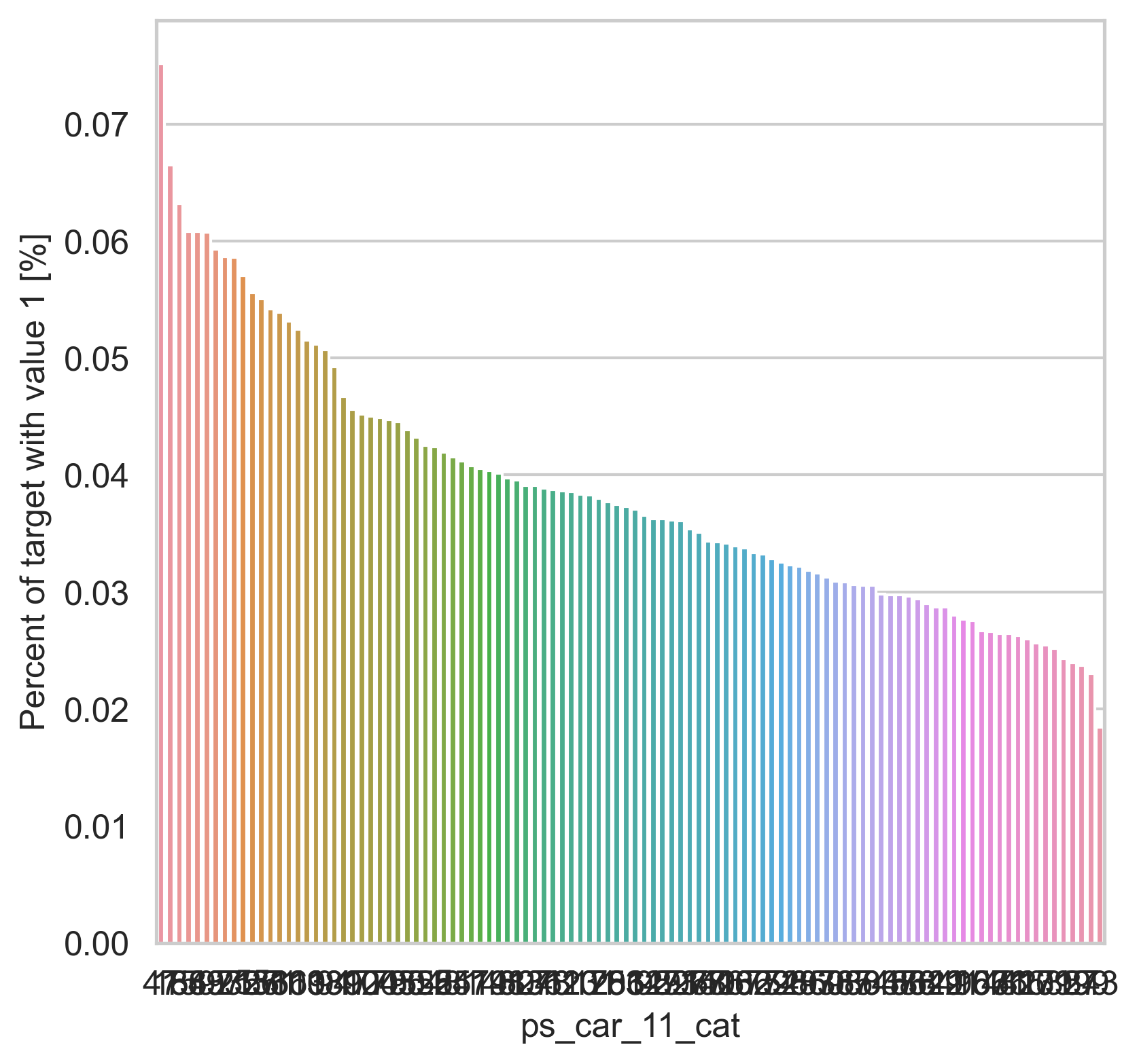
범주형 데이터에서는 두가지 방법으로 분포를 나타냅니다. 첫번째론 카테고리 값에 따른 target=1의 비율을 계산합니다. 그리고 이 퍼센티지를 barplot을 이용해 나타냅니다.

var = metadata[(metadata.type == "categorical") & (metadata.preserve)].index

for feature in var:
    fig, ax = plt.subplots(figsize=(6, 6))
    cat_perc = trainset[[feature, "target"]].groupby([feature], as_index=False).mean()
    cat_perc.sort_values(by="target", ascending=False, inplace=True)
    sns.barplot(ax=ax, x=feature, y="target", data=cat_perc, order=cat_perc[feature])
    plt.ylabel("Percent of target with value 1 [%]", fontsize=12)
    plt.xlabel(feature, fontsize=12)
    plt.tick_params(axis="both", which="major", labelsize=12)
    plt.show()

density plot으로도 시각화를 해봅니다.

var = metadata[(metadata.type == "categorical") & (metadata.preserve)].index
i = 0
t1 = trainset.loc[trainset["target"] != 0]
t0 = trainset.loc[trainset["target"] == 0]

sns.set_style("whitegrid")
plt.figure()
fig, ax = plt.subplots(4, 4, figsize=(16, 16))

for feature in var:
    i += 1
    plt.subplot(4, 4, i)
    sns.kdeplot(t1[feature], bw=0.5, label="target = 1")
    sns.kdeplot(t0[feature], bw=0.5, label="target = 0")
    plt.xlabel(feature, fontsize=12)
    plt.ylabel("Density plot", fontsize=12)
    plt.tick_params(axis="both", which="major", labelsize=12)
plt.show()

<Figure size 2400x1500 with 0 Axes>

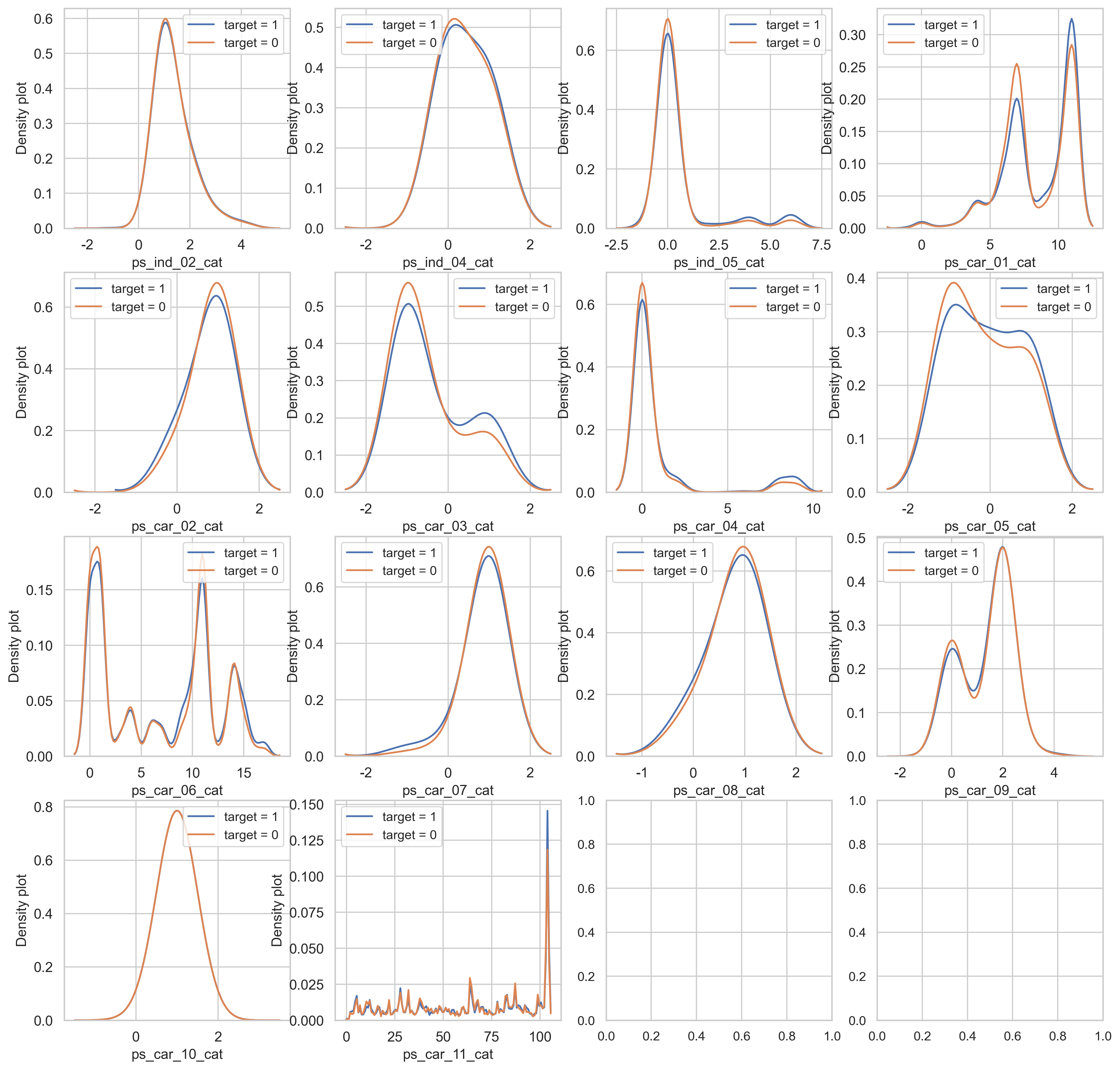
ps_car_03_cat, ps_car_05_cat 칼럼의 target=0과 target=1의 분포가 매우 다르게 보입니다.

Data unbalance between train and test data

train과 test 데이터세트를 비교해봅시다. registration feature로 시작해보겠습니다

var = metadata[(metadata.category == "registration") & (metadata.preserve)].index

sns.set_style("whitegrid")

plt.figure()
fig, ax = plt.subplots(1, 3, figsize=(12, 4))
i = 0
for feature in var:
    i += 1
    plt.subplot(1, 3, i)
    sns.kdeplot(trainset[feature], bw=0.5, label="traiin")
    sns.kdeplot(testset[feature], bw=0.5, label="test")
    plt.ylabel("Distribution", fontsize=12)
    plt.xlabel(feature, fontsize=12)
    plt.tick_params(axis="both", which="major", labelsize=12)
plt.show()

<Figure size 2400x1500 with 0 Axes>

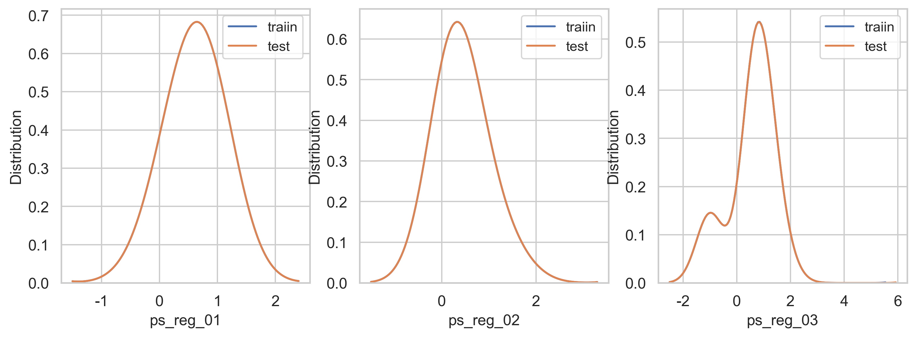
모든 reg feature는 데이터가 균형잡힌 모습입니다.

car feature을 비교해보겠습니다

var = metadata[(metadata.category == "car") & (metadata.preserve)].index

sns.set_style("whitegrid")

plt.figure()
fig, ax = plt.subplots(4, 4, figsize=(20, 16))
i = 0
for feature in var:
    i += 1
    plt.subplot(4, 4, i)
    sns.kdeplot(trainset[feature], bw=0.5, label="train")
    sns.kdeplot(testset[feature], bw=0.5, label="test")
    plt.ylabel("Distribution", fontsize=12)
    plt.xlabel(feature, fontsize=12)
    plt.tick_params(axis="both", which="major", labelsize=12)
plt.show()    

<Figure size 2400x1500 with 0 Axes>

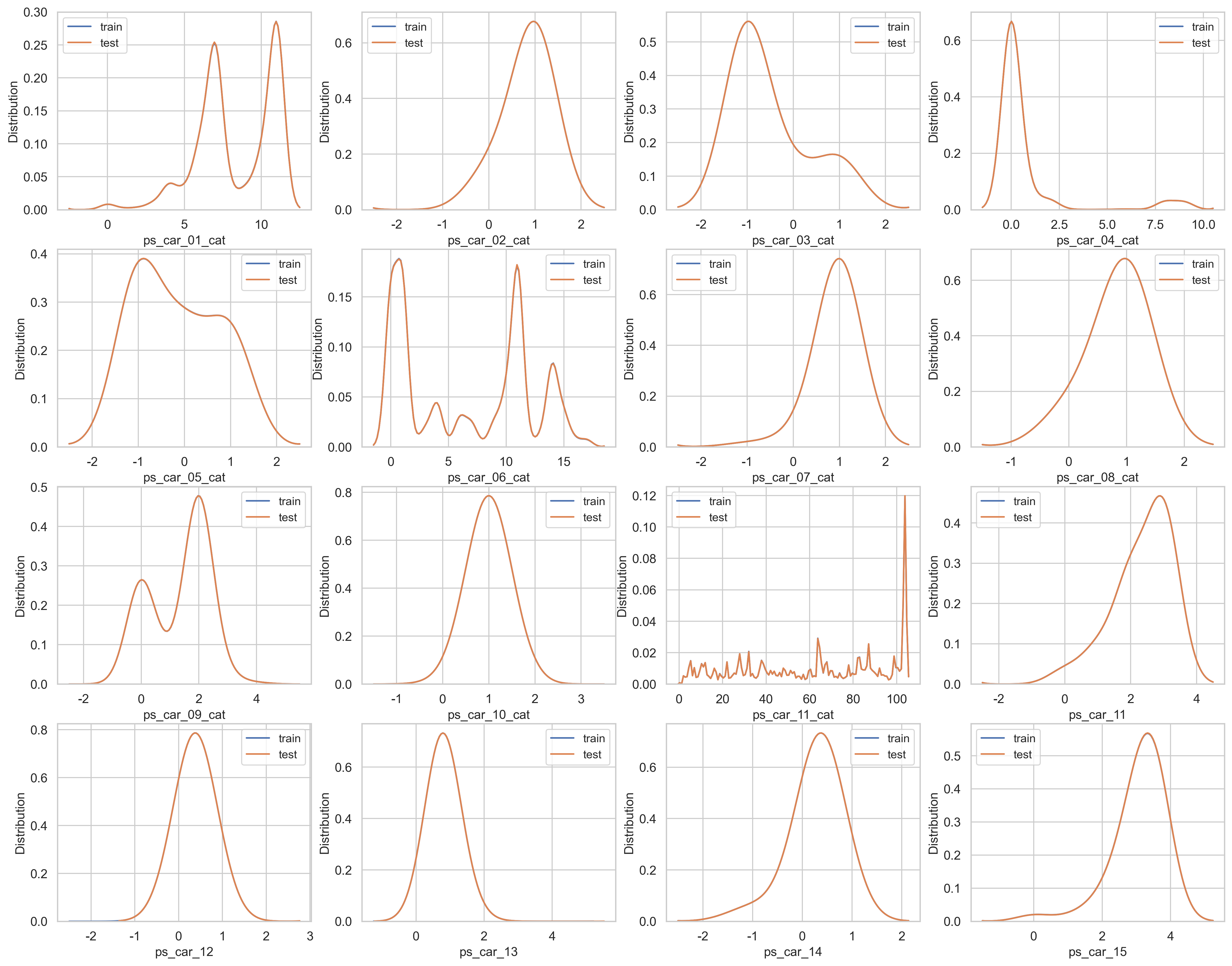
car feature 역시 모든 데이터가 균형잡힌 모습.

ind feature을 살펴봅시다.

var = metadata[(metadata.category == "individual") & (metadata.preserve)].index

sns.set_style("whitegrid")

plt.figure()
fig, ax = plt.subplots(5, 4, figsize=(20, 16))
i = 0
for feature in var:
    i += 1
    plt.subplot(5, 4, i)
    sns.kdeplot(trainset[feature], bw=0.5, label="train")
    sns.kdeplot(testset[feature], bw=0.5, label="test")
    plt.ylabel("Distribution", fontsize=12)
    plt.xlabel(feature, fontsize=12)
    plt.tick_params(axis="both", which="major", labelsize=12)
plt.show()

<Figure size 2400x1500 with 0 Axes>

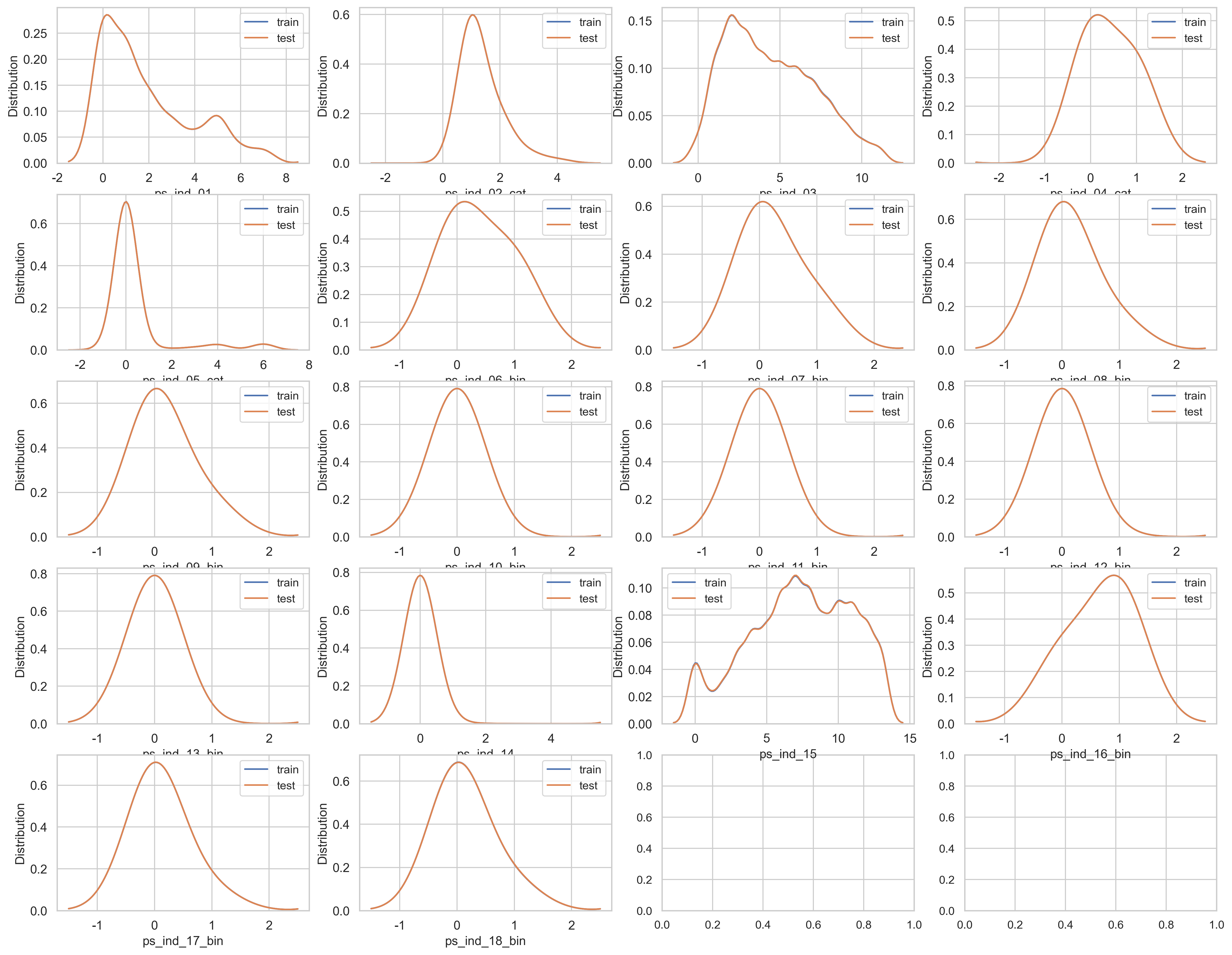
모든 ind feature 또한 데이터가 균형 잡힌 모습.

calc feature을 확인해봅시다

var = metadata[(metadata.category == "calculated") & (metadata.preserve)].index

sns.set_style("whitegrid")

plt.figure()
fig, ax = plt.subplots(5, 4, figsize=(20, 16))
i = 0
for feature in var:
    i += 1
    plt.subplot(5, 4, i)
    sns.kdeplot(trainset[feature], bw=0.5, label="train")
    sns.kdeplot(testset[feature], bw=0.5, label="test")
    plt.ylabel("Distribution", fontsize=12)
    plt.tick_params(axis="both", which="major", labelsize=12)
plt.show()

<Figure size 2400x1500 with 0 Axes>

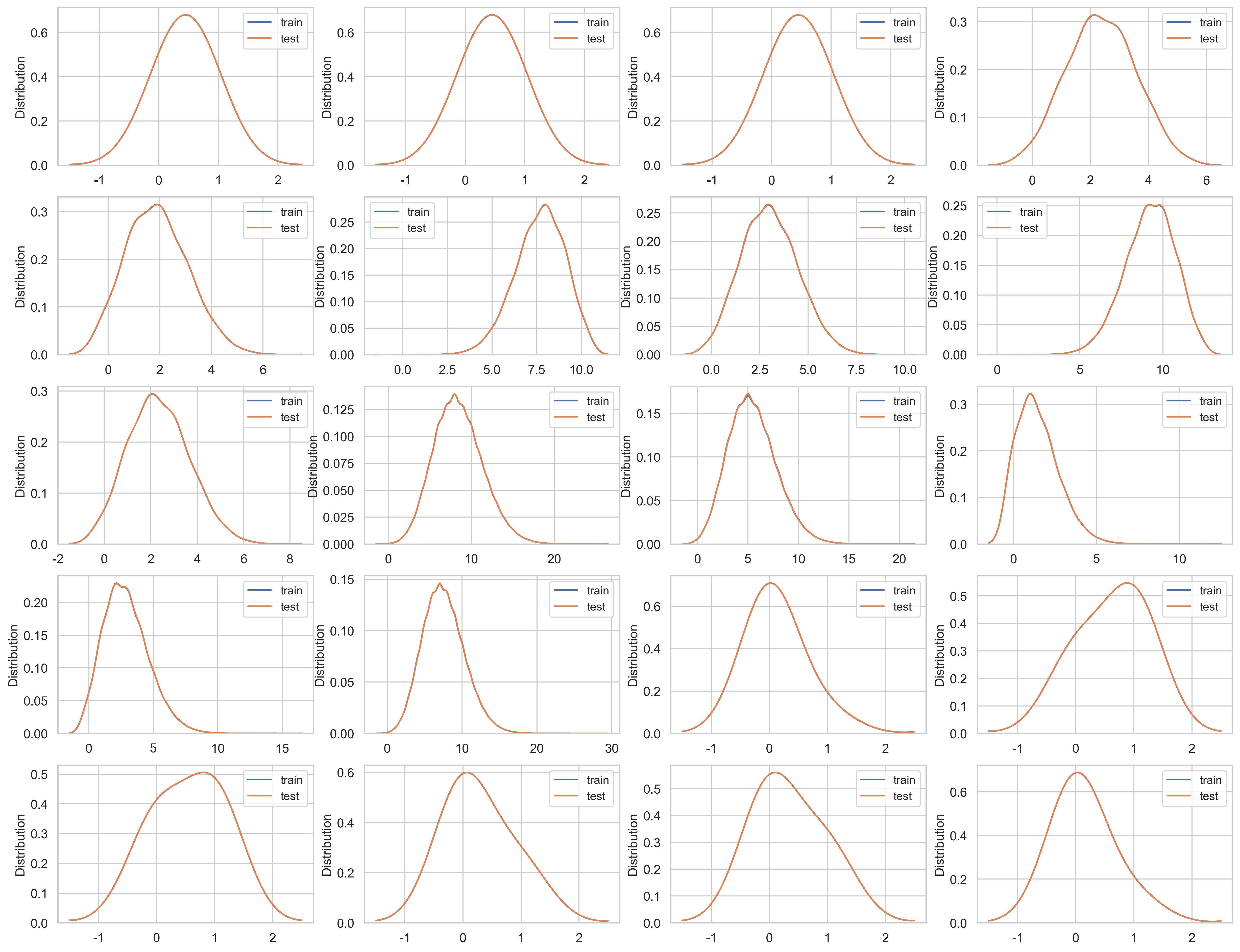
calc feature도 train과 test 데이터세트의 데이터가 균형잡힌 모습.

참고 문헌 [5]에 따르면 train과 test 데이터세트의 데이터는 균형잡힌 모습이라는 것을 확인할 수 있고, calc feature는 모두 엔지니어링되었거나 상관이 없을 수도 있다는 것을 암시합니다. 이러한 것들은 한개 이상의 예측모델로 CV score을 이용하여 신중한 연속적인 제거를 통해 평가될 수 있습니다

Check data quality

결측치를 확인해봅시다

vars_with_missing = []

for feature in trainset.columns:
    missings = trainset[trainset[feature] == -1][feature].count()
    if missings > 0:
        vars_with_missing.append(feature)
        missings_perc = missings/trainset.shape[0]
        
        print('Variable {} has {} records ({:.2%}) with missing values'.format(feature, missings, missings_perc))
        
print('In total, there are {} variables with missing values'.format(len(vars_with_missing)))

Variable ps_ind_02_cat has 216 records (0.04%) with missing values
Variable ps_ind_04_cat has 83 records (0.01%) with missing values
Variable ps_ind_05_cat has 5809 records (0.98%) with missing values
Variable ps_reg_03 has 107772 records (18.11%) with missing values
Variable ps_car_01_cat has 107 records (0.02%) with missing values
Variable ps_car_02_cat has 5 records (0.00%) with missing values
Variable ps_car_03_cat has 411231 records (69.09%) with missing values
Variable ps_car_05_cat has 266551 records (44.78%) with missing values
Variable ps_car_07_cat has 11489 records (1.93%) with missing values
Variable ps_car_09_cat has 569 records (0.10%) with missing values
Variable ps_car_11 has 5 records (0.00%) with missing values
Variable ps_car_12 has 1 records (0.00%) with missing values
Variable ps_car_14 has 42620 records (7.16%) with missing values
In total, there are 13 variables with missing values

Prepare the data for model

Drop calc columns

[5]에서의 제안에 따라, calc coluns를 제거합니다. 이 칼럼들은 모두 엔지니어링된 것으로 보이며, Dmitry Altukhov에 따르면 이 칼럼들을 제거함에 따라 그의 CV score가 개선될 수 있었다고 합니다

col_to_drop = trainset.columns[trainset.columns.str.startswith("ps_calc_")]
trainset = trainset.drop(col_to_drop, axis=1)
testset = testset.drop(col_to_drop, axis=1)

결측치가 너무 많은 feature 제거

ps_car_03_cat과 ps_car_05_cat을 제거합니다

vars_to_drop = ["ps_car_03_cat", "ps_car_05_cat"]
trainset.drop(vars_to_drop, inplace=True, axis=1)
testset.drop(vars_to_drop, inplace=True, axis=1)
metadata.loc[(vars_to_drop), "preserve"] = False # metadata 업데이트

범주형 변수 인코딩

해당 커널에서는 distinct value가 많은 ps_car_11_cat 변수들에 대해서는 mean encoding을 사용하였고, 나머지 범주형 변수들에 대해서는 더미 변수를 생성하는 one-hot encoding의 방식 사용

Mean encoding이란?

• 목표

카테고리 변수에 대하여 (여기서는 104개의 카테고리를 가진 ps_car_11_cat 변수에 대하여) 단순하게 0,1로 구분된 target값에 대한 의미를 가지도록 만드는 것

• Method

카테고리 변수의 Label 값에 따라서 Target 값의 평균을 구해 각 Label이 Target과 가지는 상관성, 영향 도출

• 문제점

1. target값을 이용해 계산하기 때문에 overfitting의 문제가 발생할 수 있음 -> 이 커널에서는 noise를 추가하는 방식으로 이 문제를 해결

2. test 데이터와 train 데이터 간의 분포가 다른 경우 (ex. 한쪽이 불균형 데이터인 경우) 이때도 마찬가지로 overfitting의 문제 발생 가능 -> Smoothing을 통해 문제 해결

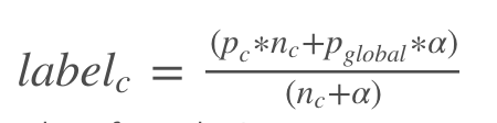
Smoothing 공식

# Script by https://www.kaggle.com/ogrellier
# Code: https://www.kaggle.com/ogrellier/python-target-encoding-for-categorical-features
def add_noise(series, noise_level):
    return series * (1 + noise_level * np.random.randn(len(series)))

def target_encode(trn_series=None,
                  tst_series=None,
                  target=None,
                  min_samples_leaf=1,
                  smoothing=1,
                  noise_level=0):
    '''
    trn_series : training categorical feature as a pd.Series
    tst_series : test categorical feature as a pd.Series
    target : target data as a pd.Series
    min_samples_leaf (int) : minimum samples to take category average into account
    smoothing (int) : smoothing effect to balance categorical average vs prior  
    '''
    
    assert len(trn_series) == len(target)
    assert trn_series.name == tst_series.name
    temp = pd.concat([trn_series, target], axis=1)
    
    # Compute target mean
    averages = temp.groupby(trn_series.name)[target.name].agg(["mean", "count"])
    
    # Compute smoothing
    # sigmoid
    smoothing = 1 / (1 + np.exp(-(averages["count"] - min_samples_leaf) / smoothing))
    
    prior = target.mean()
    
    # count가 클수록 full_avg는 적게 고려된다.
    averages[target.name] = prior * (1 - smoothing) + averages["mean"] * smoothing
    averages.drop(["mean", "count"], axis=1, inplace=True)
    
    # trn과 tst에 series에 average 적용
    ft_trn_series = pd.merge(
        trn_series.to_frame(trn_series.name),
        averages.reset_index().rename(columns={'index': target.name, target.name: 'average'}),
        on=trn_series.name,
        how='left')['average'].rename(trn_series.name + '_mean').fillna(prior)
    # pd.merge는 index를 유지하지 않으므로 저장
    ft_trn_series.index = trn_series.index 
    
    ft_tst_series = pd.merge(
        tst_series.to_frame(tst_series.name),
        averages.reset_index().rename(columns={'index': target.name, target.name: 'average'}),
        on=tst_series.name,
        how='left')['average'].rename(trn_series.name + '_mean').fillna(prior)
    # pd.merge는 index를 유지하지 않으므로 저장
    ft_tst_series.index = tst_series.index
    
    return add_noise(ft_trn_series, noise_level), add_noise(ft_tst_series, noise_level)

Replace ps_car_11_cat with encoded value

target_encode 함수를 이용하여, ps_car_11_cat의 값을 바꿔줍니다

train_encoded, test_encoded = target_encode(trainset["ps_car_11_cat"], 
                             testset["ps_car_11_cat"], 
                             target=trainset.target, 
                             min_samples_leaf=100,
                             smoothing=10,
                             noise_level=0.01)

trainset["ps_car_11_cat_te"] = train_encoded
trainset.drop("ps_car_11_cat", axis=1, inplace=True)
metadata.loc["ps_car_11_cat", "preserve"] = False
testset["ps_car_11_cat_te"] = test_encoded
testset.drop("ps_car_11_cat", axis=1, inplace=True)

Balance target variable

target 칼럼의 데이터는 매우 불균형합니다. 이러한 경우, target=0을 undersampling하거나 target=1을 oversampling하여 개선할 수 있습니다. 여기선 train set가 매우 크기 때문에 undersampling을 해줍니다.

desired_apriori = 0.1

idx_0 = trainset[trainset.target == 0].index
idx_1 = trainset[trainset.target == 1].index

nb_0 = len(trainset.loc[idx_0])
nb_1 = len(trainset.loc[idx_1])

undersampling_rate = ((1-desired_apriori) * nb_1) / (nb_0 * desired_apriori)
undersampled_nb_0 = int(undersampling_rate * nb_0)
print('Rate to undersample records with target=0: {}'.format(undersampling_rate))
print('Number of records with target=0 after undersampling: {}'.format(undersampled_nb_0))

# 언더샘플링한 개수만큼 target=0인 데이터를 랜덤으로 선택
undersampled_idx = shuffle(idx_0, random_state=314, n_samples=undersampled_nb_0)

idx_list = list(undersampled_idx) + list(idx_1)

trainset = trainset.loc[idx_list].reset_index(drop=True)

Rate to undersample records with target=0: 0.34043569687437886
Number of records with target=0 after undersampling: 195246

Replace -1 values with NaN

trainset = trainset.replace(-1, np.nan)
testset = testset.replace(-1, np.nan)

Dummify cat values

categorical (cat) 칼럼의 값들은 가변수화 해준다.

cat_features = [a for a in trainset.columns if a.endswith("cat")]

for column in cat_features:
    temp = pd.get_dummies(pd.Series(trainset[column]))
    trainset = pd.concat([trainset, temp], axis=1)
    trainset = trainset.drop([column], axis=1)
    
for column in cat_features:
    temp = pd.get_dummies(pd.Series(testset[column]))
    testset = pd.concat([testset, temp], axis=1)
    testset = testset.drop([column], axis=1)

Drop unused and target columns

id와 target 칼럼을 분리해줍니다. (이 칼럼들을 제거)

id_test = testset['id'].values
target_train = trainset['target'].values

trainset = trainset.drop(['target','id'], axis = 1)
testset = testset.drop(['id'], axis = 1)

print("Train dataset (rows, cols):",trainset.values.shape, "\nTest dataset (rows, cols):",testset.values.shape)

Train dataset (rows, cols): (216940, 91) 
Test dataset (rows, cols): (892816, 91)

Prepare the model

cross validation과 앙상블을 위한 Ensemble 클래스

4개의 변수를 가진다:

• self - 초기화할 객체
• n_splits - cross-validation 분할 수
• stacker - 학습한 모델들로부터 나온 예측 결과들을 쌓는데 사용되는 모델
• base_models - 훈련에 사용할 모델들의 리스트

두번째 메서드, fit_predict는 4개의 기능을 갖는다:

• n_splits의 개수로 training data를 나눈다
• 각각의 fold를 base models로 학습한다.
• 각각의 모델을 사용하여 예측을 수행한다.
• stacker를 이용하여 결과들을 앙상블

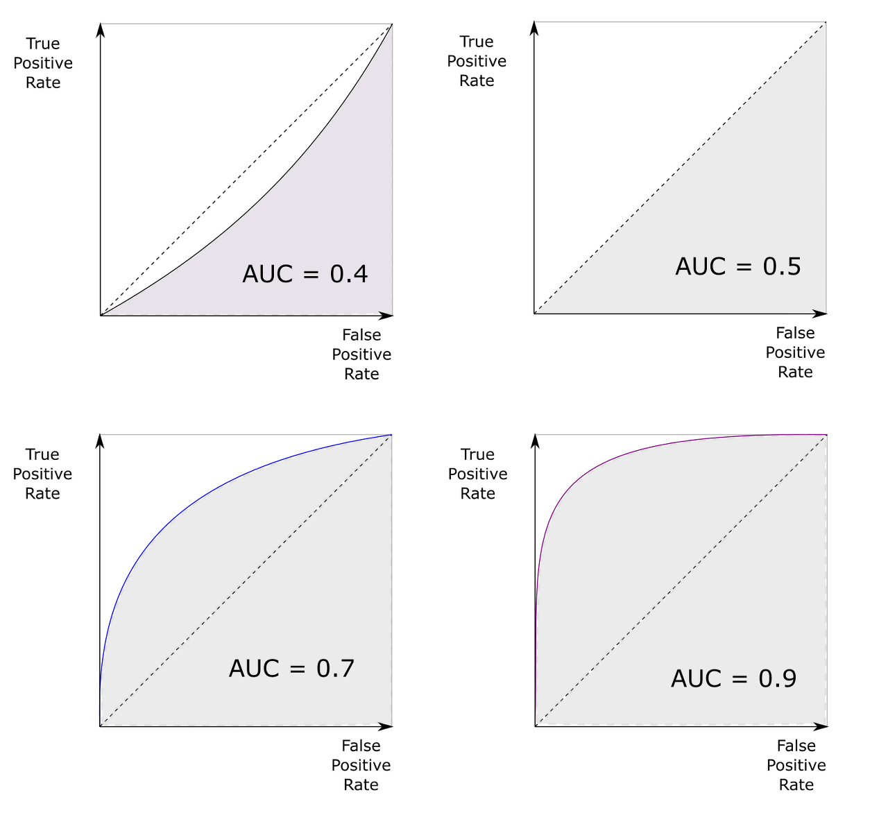
Roc 곡선과 이에 기반한 AUC 스코어:

• 타깃이 되는 특성의 클래스 레이블 분포가 불균형할 때, accuracy의 단점을 보완하면서, decision boundary에 덜 민감하게 안정적으로 label을 더 잘 분류-예측할 수 있다는 장점이 있다
• 머신러닝의 이진 분류 모델의 성능을 판단하는 중요 지표
• ROC 곡선은 FPR(x 축)이 변할 때 TPR(y 축)이 어떻게 변하는지를 나타내는 곡선.
• 1에 가까울수록 좋은 수치
• TPR = (TP / (FN + TP))
• FPR = (FP / (FP + TN))

class Ensemble(object):
    def __init__(self, n_splits, stacker, base_models):
        self.n_splits = n_splits
        self.stacker = stacker
        self.base_models = base_models
    
    def fit_predict(self, X, y, T):
        X = np.array(X)
        y = np.array(y)
        T = np.array(T)
        
        folds = list(StratifiedKFold(n_splits=self.n_splits, shuffle=True, 
                                     random_state=314).split(X, y))
        
        S_train = np.zeros((X.shape[0], len(self.base_models)))
        S_test = np.zeros((T.shape[0], len(self.base_models)))
        
        for i, clf in enumerate(self.base_models):
            S_test_i = np.zeros((T.shape[0], self.n_splits))
            for j, (train_idx, test_idx) in enumerate(folds):
                X_train = X[train_idx]
                y_train = y[train_idx]
                X_holdout = X[test_idx]
                
                print(str(clf))
                print ("Base model %d: fit %s model | fold %d" % (i+1, str(clf).split('(')[0], j+1))
                clf.fit(X_train, y_train)
                cross_score = cross_val_score(clf, X_train, y_train, cv=3, scoring="roc_auc")
                print("cross_score [roc-auc]: %.5f [gini]: %.5f" % (cross_score.mean(), 2*cross_score.mean()-1))
                
                y_pred = clf.predict_proba(X_holdout)[:, 1] # return: (n_samples, n_classes)
                S_train[test_idx, i] = y_pred
                S_test_i[:, j] = clf.predict_proba(T)[:, 1]
            S_test[:, i] = S_test_i.mean(axis=1)
            
        results = cross_val_score(self.stacker, S_train, y, cv=3, scoring="roc_auc")
        # Calculate gini factor as 2 * AUC - 1
        print("Stacker score [gini]: %.5f" % (2 * results.mean() - 1))
        self.stacker.fit(S_train, y)
        res = self.stacker.predict_proba(S_test)[:, 1]
        return res

Parameters for the base models

3개의 다른 LightGBM 모델과 XGB 모델을 사용합니다

# LightGBM params
# lgb_1
lgb_params1 = {}
lgb_params1['learning_rate'] = 0.02
lgb_params1['n_estimators'] = 650
lgb_params1['max_bin'] = 10
lgb_params1['subsample'] = 0.8
lgb_params1['subsample_freq'] = 10
lgb_params1['colsample_bytree'] = 0.8   
lgb_params1['min_child_samples'] = 500
lgb_params1['seed'] = 314
lgb_params1['num_threads'] = 4

# lgb2
lgb_params2 = {}
lgb_params2['n_estimators'] = 1090
lgb_params2['learning_rate'] = 0.02
lgb_params2['colsample_bytree'] = 0.3   
lgb_params2['subsample'] = 0.7
lgb_params2['subsample_freq'] = 2
lgb_params2['num_leaves'] = 16
lgb_params2['seed'] = 314
lgb_params2['num_threads'] = 4

# lgb3
lgb_params3 = {}
lgb_params3['n_estimators'] = 1100
lgb_params3['max_depth'] = 4
lgb_params3['learning_rate'] = 0.02
lgb_params3['seed'] = 314
lgb_params3['num_threads'] = 4

# XGBoost params
xgb_params = {}
xgb_params['objective'] = 'binary:logistic'
xgb_params['learning_rate'] = 0.04
xgb_params['n_estimators'] = 490
xgb_params['max_depth'] = 4
xgb_params['subsample'] = 0.9
xgb_params['colsample_bytree'] = 0.9  
xgb_params['min_child_weight'] = 10
xgb_params['num_threads'] = 4

Initialize the models with the parameters

# Base models
lgb_model1 = LGBMClassifier(**lgb_params1)

lgb_model2 = LGBMClassifier(**lgb_params2)
       
lgb_model3 = LGBMClassifier(**lgb_params3)

xgb_model = XGBClassifier(**xgb_params)

# Stacking model
log_model = LogisticRegression()

Initialize the ensambling object

stack = Ensemble(n_splits=3, stacker=log_model, 
                 base_models=(lgb_model1, lgb_model2, lgb_model3, xgb_model))  

Run the predictive models

y_prediction = stack.fit_predict(trainset, target_train, testset)

LGBMClassifier(colsample_bytree=0.8, learning_rate=0.02, max_bin=10,
               min_child_samples=500, n_estimators=650, num_threads=4, seed=314,
               subsample=0.8, subsample_freq=10)
Base model 1: fit LGBMClassifier model | fold 1

Base model 1: fit LGBMClassifier model | fold 2

Base model 1: fit LGBMClassifier model | fold 3

Base model 2: fit LGBMClassifier model | fold 1

cross_score [roc-auc]: 0.63938 [gini]: 0.27875
Base model 2: fit LGBMClassifier model | fold 2
[LightGBM] [Warning] num_threads is set=4, n_jobs=-1 will be ignored. Current value: num_threads=4
[LightGBM] [Warning] num_threads is set=4, n_jobs=-1 will be ignored. Current value: num_threads=4
[LightGBM] [Warning] num_threads is set=4, n_jobs=-1 will be ignored. Current value: num_threads=4
cross_score [roc-auc]: 0.63993 [gini]: 0.27987
LGBMClassifier(colsample_bytree=0.3, learning_rate=0.02, n_estimators=1090,
               num_leaves=16, num_threads=4, seed=314, subsample=0.7,
               subsample_freq=2)
Base model 2: fit LGBMClassifier model | fold 3
[LightGBM] [Warning] num_threads is set=4, n_jobs=-1 will be ignored. Current value: num_threads=4
[LightGBM] [Warning] num_threads is set=4, n_jobs=-1 will be ignored. Current value: num_threads=4
[LightGBM] [Warning] num_threads is set=4, n_jobs=-1 will be ignored. Current value: num_threads=4
cross_score [roc-auc]: 0.63792 [gini]: 0.27585
LGBMClassifier(learning_rate=0.02, max_depth=4, n_estimators=1100,
               num_threads=4, seed=314)
Base model 3: fit LGBMClassifier model | fold 1
[LightGBM] [Warning] num_threads is set=4, n_jobs=-1 will be ignored. Current value: num_threads=4
[LightGBM] [Warning] num_threads is set=4, n_jobs=-1 will be ignored. Current value: num_threads=4
[LightGBM] [Warning] num_threads is set=4, n_jobs=-1 will be ignored. Current value: num_threads=4
cross_score [roc-auc]: 0.63657 [gini]: 0.27314
LGBMClassifier(learning_rate=0.02, max_depth=4, n_estimators=1100,
               num_threads=4, seed=314)
Base model 3: fit LGBMClassifier model | fold 2
[LightGBM] [Warning] num_threads is set=4, n_jobs=-1 will be ignored. Current value: num_threads=4
[LightGBM] [Warning] num_threads is set=4, n_jobs=-1 will be ignored. Current value: num_threads=4
[LightGBM] [Warning] num_threads is set=4, n_jobs=-1 will be ignored. Current value: num_threads=4
cross_score [roc-auc]: 0.63709 [gini]: 0.27417
LGBMClassifier(learning_rate=0.02, max_depth=4, n_estimators=1100,
               num_threads=4, seed=314)
Base model 3: fit LGBMClassifier model | fold 3
[LightGBM] [Warning] num_threads is set=4, n_jobs=-1 will be ignored. Current value: num_threads=4
[LightGBM] [Warning] num_threads is set=4, n_jobs=-1 will be ignored. Current value: num_threads=4
[LightGBM] [Warning] num_threads is set=4, n_jobs=-1 will be ignored. Current value: num_threads=4
cross_score [roc-auc]: 0.63374 [gini]: 0.26747
XGBClassifier(base_score=None, booster=None, colsample_bylevel=None,
              colsample_bynode=None, colsample_bytree=0.9,
              enable_categorical=False, gamma=None, gpu_id=None,
              importance_type=None, interaction_constraints=None,
              learning_rate=0.04, max_delta_step=None, max_depth=4,
              min_child_weight=10, missing=nan, monotone_constraints=None,
              n_estimators=490, n_jobs=None, num_parallel_tree=None,
              num_threads=4, predictor=None, random_state=None, reg_alpha=None,
              reg_lambda=None, scale_pos_weight=None, subsample=0.9,
              tree_method=None, validate_parameters=None, verbosity=None)
Base model 4: fit XGBClassifier model | fold 1
[21:00:40] WARNING: C:/Users/Administrator/workspace/xgboost-win64_release_1.5.1/src/learner.cc:576: 
Parameters: { "num_threads" } might not be used.

  This could be a false alarm, with some parameters getting used by language bindings but
  then being mistakenly passed down to XGBoost core, or some parameter actually being used
  but getting flagged wrongly here. Please open an issue if you find any such cases.


[21:00:40] WARNING: C:/Users/Administrator/workspace/xgboost-win64_release_1.5.1/src/learner.cc:1115: Starting in XGBoost 1.3.0, the default evaluation metric used with the objective 'binary:logistic' was changed from 'error' to 'logloss'. Explicitly set eval_metric if you'd like to restore the old behavior.
[21:01:10] WARNING: C:/Users/Administrator/workspace/xgboost-win64_release_1.5.1/src/learner.cc:576: 
Parameters: { "num_threads" } might not be used.

  This could be a false alarm, with some parameters getting used by language bindings but
  then being mistakenly passed down to XGBoost core, or some parameter actually being used
  but getting flagged wrongly here. Please open an issue if you find any such cases.


[21:01:10] WARNING: C:/Users/Administrator/workspace/xgboost-win64_release_1.5.1/src/learner.cc:1115: Starting in XGBoost 1.3.0, the default evaluation metric used with the objective 'binary:logistic' was changed from 'error' to 'logloss'. Explicitly set eval_metric if you'd like to restore the old behavior.
[21:01:31] WARNING: C:/Users/Administrator/workspace/xgboost-win64_release_1.5.1/src/learner.cc:576: 
Parameters: { "num_threads" } might not be used.

  This could be a false alarm, with some parameters getting used by language bindings but
  then being mistakenly passed down to XGBoost core, or some parameter actually being used
  but getting flagged wrongly here. Please open an issue if you find any such cases.


[21:01:31] WARNING: C:/Users/Administrator/workspace/xgboost-win64_release_1.5.1/src/learner.cc:1115: Starting in XGBoost 1.3.0, the default evaluation metric used with the objective 'binary:logistic' was changed from 'error' to 'logloss'. Explicitly set eval_metric if you'd like to restore the old behavior.
[21:01:52] WARNING: C:/Users/Administrator/workspace/xgboost-win64_release_1.5.1/src/learner.cc:576: 
Parameters: { "num_threads" } might not be used.

  This could be a false alarm, with some parameters getting used by language bindings but
  then being mistakenly passed down to XGBoost core, or some parameter actually being used
  but getting flagged wrongly here. Please open an issue if you find any such cases.


[21:01:52] WARNING: C:/Users/Administrator/workspace/xgboost-win64_release_1.5.1/src/learner.cc:1115: Starting in XGBoost 1.3.0, the default evaluation metric used with the objective 'binary:logistic' was changed from 'error' to 'logloss'. Explicitly set eval_metric if you'd like to restore the old behavior.
cross_score [roc-auc]: 0.63873 [gini]: 0.27746
XGBClassifier(base_score=0.5, booster='gbtree', colsample_bylevel=1,
              colsample_bynode=1, colsample_bytree=0.9,
              enable_categorical=False, gamma=0, gpu_id=-1,
              importance_type=None, interaction_constraints='',
              learning_rate=0.04, max_delta_step=0, max_depth=4,
              min_child_weight=10, missing=nan, monotone_constraints='()',
              n_estimators=490, n_jobs=6, num_parallel_tree=1, num_threads=4,
              predictor='auto', random_state=0, reg_alpha=0, reg_lambda=1,
              scale_pos_weight=1, subsample=0.9, tree_method='exact',
              validate_parameters=1, verbosity=None)
Base model 4: fit XGBClassifier model | fold 2
[21:02:14] WARNING: C:/Users/Administrator/workspace/xgboost-win64_release_1.5.1/src/learner.cc:576: 
Parameters: { "num_threads" } might not be used.

  This could be a false alarm, with some parameters getting used by language bindings but
  then being mistakenly passed down to XGBoost core, or some parameter actually being used
  but getting flagged wrongly here. Please open an issue if you find any such cases.


[21:02:14] WARNING: C:/Users/Administrator/workspace/xgboost-win64_release_1.5.1/src/learner.cc:1115: Starting in XGBoost 1.3.0, the default evaluation metric used with the objective 'binary:logistic' was changed from 'error' to 'logloss'. Explicitly set eval_metric if you'd like to restore the old behavior.
[21:02:45] WARNING: C:/Users/Administrator/workspace/xgboost-win64_release_1.5.1/src/learner.cc:576: 
Parameters: { "num_threads" } might not be used.

  This could be a false alarm, with some parameters getting used by language bindings but
  then being mistakenly passed down to XGBoost core, or some parameter actually being used
  but getting flagged wrongly here. Please open an issue if you find any such cases.


[21:02:45] WARNING: C:/Users/Administrator/workspace/xgboost-win64_release_1.5.1/src/learner.cc:1115: Starting in XGBoost 1.3.0, the default evaluation metric used with the objective 'binary:logistic' was changed from 'error' to 'logloss'. Explicitly set eval_metric if you'd like to restore the old behavior.
[21:03:06] WARNING: C:/Users/Administrator/workspace/xgboost-win64_release_1.5.1/src/learner.cc:576: 
Parameters: { "num_threads" } might not be used.

  This could be a false alarm, with some parameters getting used by language bindings but
  then being mistakenly passed down to XGBoost core, or some parameter actually being used
  but getting flagged wrongly here. Please open an issue if you find any such cases.


[21:03:06] WARNING: C:/Users/Administrator/workspace/xgboost-win64_release_1.5.1/src/learner.cc:1115: Starting in XGBoost 1.3.0, the default evaluation metric used with the objective 'binary:logistic' was changed from 'error' to 'logloss'. Explicitly set eval_metric if you'd like to restore the old behavior.
[21:03:29] WARNING: C:/Users/Administrator/workspace/xgboost-win64_release_1.5.1/src/learner.cc:576: 
Parameters: { "num_threads" } might not be used.

  This could be a false alarm, with some parameters getting used by language bindings but
  then being mistakenly passed down to XGBoost core, or some parameter actually being used
  but getting flagged wrongly here. Please open an issue if you find any such cases.


[21:03:29] WARNING: C:/Users/Administrator/workspace/xgboost-win64_release_1.5.1/src/learner.cc:1115: Starting in XGBoost 1.3.0, the default evaluation metric used with the objective 'binary:logistic' was changed from 'error' to 'logloss'. Explicitly set eval_metric if you'd like to restore the old behavior.
cross_score [roc-auc]: 0.63933 [gini]: 0.27867
XGBClassifier(base_score=0.5, booster='gbtree', colsample_bylevel=1,
              colsample_bynode=1, colsample_bytree=0.9,
              enable_categorical=False, gamma=0, gpu_id=-1,
              importance_type=None, interaction_constraints='',
              learning_rate=0.04, max_delta_step=0, max_depth=4,
              min_child_weight=10, missing=nan, monotone_constraints='()',
              n_estimators=490, n_jobs=6, num_parallel_tree=1, num_threads=4,
              predictor='auto', random_state=0, reg_alpha=0, reg_lambda=1,
              scale_pos_weight=1, subsample=0.9, tree_method='exact',
              validate_parameters=1, verbosity=None)
Base model 4: fit XGBClassifier model | fold 3
[21:03:50] WARNING: C:/Users/Administrator/workspace/xgboost-win64_release_1.5.1/src/learner.cc:576: 
Parameters: { "num_threads" } might not be used.

  This could be a false alarm, with some parameters getting used by language bindings but
  then being mistakenly passed down to XGBoost core, or some parameter actually being used
  but getting flagged wrongly here. Please open an issue if you find any such cases.


[21:03:51] WARNING: C:/Users/Administrator/workspace/xgboost-win64_release_1.5.1/src/learner.cc:1115: Starting in XGBoost 1.3.0, the default evaluation metric used with the objective 'binary:logistic' was changed from 'error' to 'logloss'. Explicitly set eval_metric if you'd like to restore the old behavior.
[21:04:21] WARNING: C:/Users/Administrator/workspace/xgboost-win64_release_1.5.1/src/learner.cc:576: 
Parameters: { "num_threads" } might not be used.

  This could be a false alarm, with some parameters getting used by language bindings but
  then being mistakenly passed down to XGBoost core, or some parameter actually being used
  but getting flagged wrongly here. Please open an issue if you find any such cases.


[21:04:21] WARNING: C:/Users/Administrator/workspace/xgboost-win64_release_1.5.1/src/learner.cc:1115: Starting in XGBoost 1.3.0, the default evaluation metric used with the objective 'binary:logistic' was changed from 'error' to 'logloss'. Explicitly set eval_metric if you'd like to restore the old behavior.
[21:04:43] WARNING: C:/Users/Administrator/workspace/xgboost-win64_release_1.5.1/src/learner.cc:576: 
Parameters: { "num_threads" } might not be used.

  This could be a false alarm, with some parameters getting used by language bindings but
  then being mistakenly passed down to XGBoost core, or some parameter actually being used
  but getting flagged wrongly here. Please open an issue if you find any such cases.


[21:04:43] WARNING: C:/Users/Administrator/workspace/xgboost-win64_release_1.5.1/src/learner.cc:1115: Starting in XGBoost 1.3.0, the default evaluation metric used with the objective 'binary:logistic' was changed from 'error' to 'logloss'. Explicitly set eval_metric if you'd like to restore the old behavior.
[21:05:03] WARNING: C:/Users/Administrator/workspace/xgboost-win64_release_1.5.1/src/learner.cc:576: 
Parameters: { "num_threads" } might not be used.

  This could be a false alarm, with some parameters getting used by language bindings but
  then being mistakenly passed down to XGBoost core, or some parameter actually being used
  but getting flagged wrongly here. Please open an issue if you find any such cases.


[21:05:03] WARNING: C:/Users/Administrator/workspace/xgboost-win64_release_1.5.1/src/learner.cc:1115: Starting in XGBoost 1.3.0, the default evaluation metric used with the objective 'binary:logistic' was changed from 'error' to 'logloss'. Explicitly set eval_metric if you'd like to restore the old behavior.
cross_score [roc-auc]: 0.63644 [gini]: 0.27289
Stacker score [gini]: 0.28494

Prepare the submission

submission = pd.DataFrame()
submission["id"] = id_test
submission["target"] = y_prediction
submission.to_csv("stacked.csv", index=False)

References

[1] Porto Seguro Safe Driver Prediction, Kaggle Competition, https://www.kaggle.com/c/porto-seguro-safe-driver-prediction
[2] Bert Carremans, Data Preparation and Exploration, Kaggle Kernel, https://www.kaggle.com/bertcarremans/data-preparation-exploration
[3] Head or Tails, Steering Whell of Fortune - Porto Seguro EDA, Kaggle Kernel, https://www.kaggle.com/headsortails/steering-wheel-of-fortune-porto-seguro-eda
[4] Anisotropic, Interactive Porto Insights - A Plot.ly Tutorial, Kaggle Kernel, https://www.kaggle.com/arthurtok/interactive-porto-insights-a-plot-ly-tutorial
[5] Dmitry Altukhov, Kaggle Porto Seguro’s Safe Driver Prediction (3rd place solution), https://www.youtube.com/watch?v=mbxZ_zqHV9c
[6] Vladimir Demidov, Simple Staker LB 0.284, https://www.kaggle.com/yekenot/simple-stacker-lb-0-284
[7] Anisotropic, Introduction to Ensembling/Stacking in Python, https://www.kaggle.com/arthurtok/introduction-to-ensembling-stacking-in-python